Information Technology Reference
In-Depth Information
6
6
5
5
4
4
3
3
0
A
6
2
2
1
5
2
1
1
4
3
4
0
3
0
O
O
1
5
1
2
2
6
2
1
3
3
7
B
4
4
8
0
5
9
5
6
6
10
7
C
7
8
8
9
9
10
10
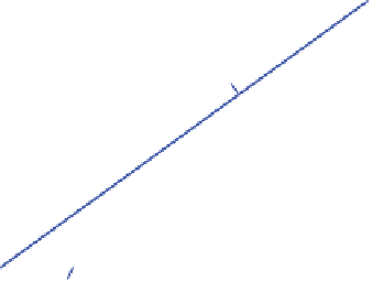
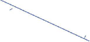
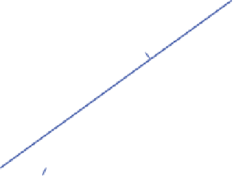
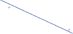
Figure 2.24
In the left-hand drawing, the black interpolative axes A, B and C intersect
at an origin O that corresponds to ugly calibrated values. It is decided to translate the
axes to intersect at the zero point on each axis. The intersection is at the centroid of the
zero points on the original axes, shown as the vertices of a dashed triangle. Each axis is
translated obliquely by the displacements shown by the arrow-headed vector to give new
parallel axes A, B and C. This looks a complicated process but the result is the simple
diagram shown in the right-hand drawing. The original origin O is retained for reasons
discussed in the main text. Sample points are not shown; their positions relative to O are
not changed by the oblique translation of the axes.
and
b
=
−
1
U
x
∗
. Clearly,
x
∗
may be replaced in (2.20) by any number of new columns
and, in particular, replacing
x
∗
by
X
gives
JB
:
p
×
p
=
J
−
1
U
X
=
J
−
1
U
U
V
=
JV
showing that the regression method correctly derives the appropriate biplot axes for the
primary data. Thus, the vector
Jb
acts similarly to a column of
VJ
and hopefully it will
be acceptable when
x
∗
refers to one or more entirely new variables. We will see during
the course of this topic that the regression method is available in other contexts (e.g.
correspondence analysis and multidimensional scaling). We note that (2.19), equivalently
(2.20), are examples of a
transition formula
, that relates samples to variables (see corre-
spondence analysis). Examples of adding variables using the regression method are given
in Chapter 3 after a discussion of the concept of axis predictivity for PCA biplots.