Solid-Fuel Rocket Motor Efficiency Improvement Scheme - Novel Combustion Concepts for Sustainable Energy Development - page 534

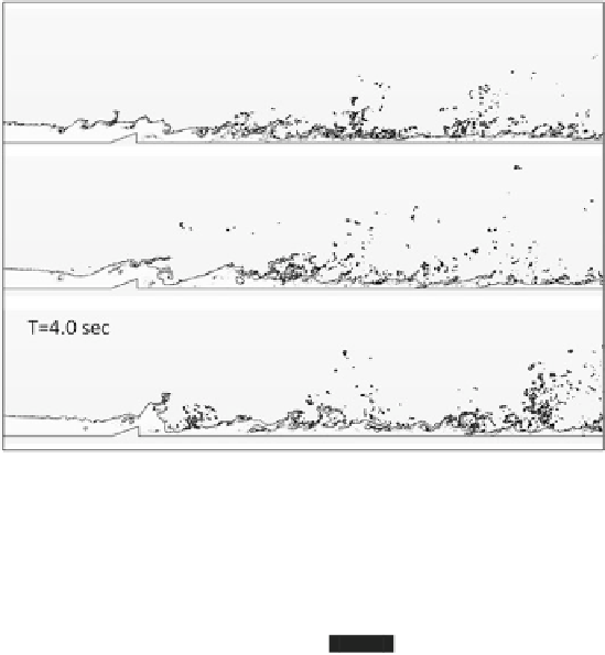
6.3 Time Averaging Boundary Length

Two-phase turbulent fl flows behave highly irregular and it is hard to capture a certain

repeatable flow pattern. Figure 6 illustrates the simulation results with the same

boundary condition and the numerical model setting over a period of different time
step, the simulation condition detail as shown in Table 2 . The breakup droplet size
might be similar in their size; however, the similarity character is dif

fl

cult to
determine from those three figures even though the operating conditions are the
same. Therefore, a method of

figure superposition is introduced in this paper in
order to visualize time-averaged contour through the results of all time steps.
In this demo (Table 3 ; Figs. 7 , 8 and 9 ), three pictures with black and white
pixels with pixel labels of 0 and 1 are shown in Fig. 7 , where pixel value 0
represents pure black and pixel value 1 represents pure white color, the illustration
of the grayscale map from corresponding pixel label value are shown in Table 3 .
The pixel superimposition is shown in Fig. 7 . After superimposition of Fig. 7 a c,

-

Fig. 6 VF of fluid boundary at different time step

Table 3 Grayscale color map

Pixel label value Gra y scale color map

0.00
0.33
0.50
0.67
1.00