A major reason for the design of multi-frequency receivers is to allow estimation and compensation of the ionospheric delay.
Simultaneous L1 and L2 pseudorange observables from the same satellite and receiver can be modeled as
where![]() is the lumped common mode errors other that the ionospheric delay
is the lumped common mode errors other that the ionospheric delay![]() represents the sum of the receiver noise and multipath errors, and
represents the sum of the receiver noise and multipath errors, and![]() and
and![]() are the carrier frequencies. In the analysis to follow, we will assume that
are the carrier frequencies. In the analysis to follow, we will assume that![]() are independent, Gaussian random variables with variance
are independent, Gaussian random variables with variance![]()
Eqns. (8.83-8.84) can be manipulated to provide an ionospheric free pseudorange observable as
which has the measurement model
Eqn. (8.85) is not usually used directly, because as shown in eqn.(8.86), the noise variance (i.e., effect of![]() is approximately
is approximately![]() The following two paragraphs discuss alternative approaches to the construction of ionospheric free pseudorange observables.
The following two paragraphs discuss alternative approaches to the construction of ionospheric free pseudorange observables.
An estimate of the ionospheric delay can be computed as
Direct substitution of eqns. (8.83-8.84) into eqn. (8.87) shows that
which shows that![]() is unbiased. The variance of
is unbiased. The variance of![]() at each epoch is approximately
at each epoch is approximately![]() Because of the magnification of the receiver noise, the ionospheric estimate of eqn. (8.87) is not used directly to compensate the pseudorange measurement. Instead, because
Because of the magnification of the receiver noise, the ionospheric estimate of eqn. (8.87) is not used directly to compensate the pseudorange measurement. Instead, because![]() changes slowly with a correlationtime of a few hours, while
changes slowly with a correlationtime of a few hours, while![]() have much shorter correlation times,
have much shorter correlation times,![]() could for example be low pass filtered by a filter with a time constant of several minutes to greatly decrease the effect of
could for example be low pass filtered by a filter with a time constant of several minutes to greatly decrease the effect of![]() while maintaining the time variation of
while maintaining the time variation of![]() If we denote the filtered version of
If we denote the filtered version of ![]() then an ionosphere free pseudorange can be computed as
then an ionosphere free pseudorange can be computed as 
which has the error model
where the ionospheric error has been (essentially) removed and the measurement noise has not been amplified. The remaining common-mode errors could be removed via differential processing. Another approach is discussed subsequently.
Simultaneous L1 and L2 phase observables from the same satellite and receiver can be modeled as
where![]() are the wavelength of the L1 and L2 carrier signals, respectively, and
are the wavelength of the L1 and L2 carrier signals, respectively, and![]() is the combined effect of multipath and receiver noise. The subsequent analysis assumes that /
is the combined effect of multipath and receiver noise. The subsequent analysis assumes that /![]() are independent Gaussian processes with variance
are independent Gaussian processes with variance![]() Using the phase observables, the ionospheric delay can be estimated as
Using the phase observables, the ionospheric delay can be estimated as
Direct substitution of eqns. (8.91) and (8.92) into eqn. (8.93) shows that
Therefore, the variance of![]() at each epoch is approximately
at each epoch is approximately![]() however, the estimate contains the significant constant bias
however, the estimate contains the significant constant bias
Eqns. (8.89) and (8.95) have the form
Eqns. (8.96) and (8.97) are in the exact form considered in Example 5.4. Therefore, the solution is
where
starting at k =1 with .![]() The estimation error variance for
The estimation error variance for![]() is
is
![]() and for
and for![]() where
where![]() and
and![]() is the ratio of the phase noise to the pseudorange noise.
is the ratio of the phase noise to the pseudorange noise.
The desire to estimate the ionospheric delay was a primary motivation for the GPS system to incorporate signals on two frequencies. The specification of the two frequencies involved a tradeoff related to the frequency spacing. If the frequency separation was too small, then measurement errors would be significantly magnified as shown in eqn. (8.88) and (8.94). However, if the frequency separation were too large, then separate antennas would be required to receive the two signals.
Wide and Narrow Lane Observables
This section develops the equations for the narrow-lane and wide-lane observables. These variables are synthesized as linear combinations of the L1 and L2 measurements. The interest in the wide-lane signal is that its wavelength is large enough that the wide-lane variable is often used to facilitate the problem of integer ambiguity resolution, see Section 8.9.
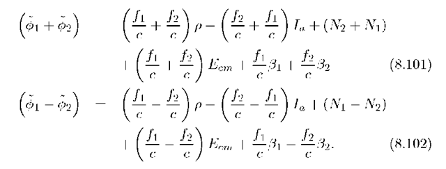
The phase measurements of eqns. (8.91-8.92) can be modeled as
Forming the sum and difference of eqns. (8.99) and (8.100) results in
By defining the wide and narrow lane wavelengths as
eqns. (8.101) and (8.102) can be written in meters as
where![]() therefore, the standard deviation of the widelane noise
therefore, the standard deviation of the widelane noise![]() is approximately 5.7 times the standard deviation of the L1 or L2 phase noise
is approximately 5.7 times the standard deviation of the L1 or L2 phase noise![]() The fact that the wide-lane phase has a wavelength of approximately 86cm can simplify integer ambiguity resolution in differential GPS applications. The pseudorange estimates can be processed similarly yielding
The fact that the wide-lane phase has a wavelength of approximately 86cm can simplify integer ambiguity resolution in differential GPS applications. The pseudorange estimates can be processed similarly yielding
Both the code and phase narrow-lane observables have noise reduced by![]()


