Abstract
The basic rules of balancing the expected return on an investment against its contribution to portfolio risk are surveyed. The related concept of Capital Asset Pricing Model asserting that the expected return of an asset must be linearly related to the covariance of its return with the return of the market portfolio if the market is efficient and its statistical tests in terms of Arbitraging Price Theory are also surveyed. The intertemporal generalization and issues of estimation errors and portfolio choice are discussed as well.
Introduction
Stock prices are volatile. The more volatile a stock, the more uncertain its future value. Investment success depends on being prepared for and being willing to take risk. The insights provided by modern portfolio theory arise from the interplay between the mathematics of return and risk. The central theme of modern portfolio theory is: ”In constructing their portfolios investors need to look at the expected return of each investment in relation to the impact that it has on the risk of the overall portfolio” (Litterman et al., 2003).
To balance the expected return of an investment against its contribution to portfolio risk, an investment’s contribution to portfolio risk is not just the risk of the investment itself, but rather the degree to which the value of that investment moves up and down with the values of the other investments in the portfolio. This degree to which these returns move together is measured by the statistical quantity called ”covariance,” which is itself a function of their correlation along with their volatilities when volatility of a stock is measured by its standard deviation (square root of variance). However, covariances are not observed directly; they are inferred from statistics that are notoriously unstable.
In Section 19.2, we summarize the Markowitz (1952, 1959) mean-variance allocations rule under the assumption that the correlations and volatilities of investment returns are known. Section 19.3 describes the relationship between the mean variance efficiency and asset pricing models. Section 19.4 discusses issues of estimation in portfolio selection.
Mean-Variance Portfolio Selection
The basic portfolio theory is normative. It considers efficient techniques for selecting portfolios based on predicted performance of individual securities. Marschak (1938) was the first to express preference in terms of indifference curves in a mean-variance space. Von Neumann and Morgen-stern (1947) provided an axiomatic framework to study the theory of choice under uncertainty. Based on these developments, Markowitz (1952, 1959) developed a mean-variance approach of asset allocation.
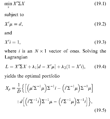
Suppose there are N securities indexed by i, i = 1,…, N. Let R’ = (R1,…, RN) denote the return of these N securities. Let m = ER and S be the mean and the nonsingular covariance matrix of R. A portfolio is described by an allocation vector X’ = (x1,…, xN) of quantity xi for the ith security. In the mean-variance approach, an investor selects the composition of the portfolio to maximize her expected return while minimizing the risk (i.e. the variance) subject to budget constraint. Since these objectives are contradictory, the investor compromises and selects the portfolio that minimizes the risk subject to a given expected return, say d. A portfolio X is said to be the minimum-variance portfolio of all portfolios with mean (or expected) return d if its portfolio weight vector is the solution to the following constrained minimization:
From Equation (19.5), we have:
Proposition 1: Any two distinct minimum-variance portfolios can generate the minimum variance frontier.
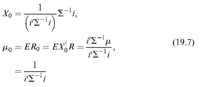
Proposition 2: Let portfolio o as the portfolio with the smallest possible variance for any mean return, then the global minimum variance portfolio has
Proposition 3: The covariance of the return of the global minimum-variance portfolio o with any portfolio p is
that is, the correlation of them is positive, corr(R0, Rp) > 0 for any portfolio p.
Proposition 4: If the covariance of the returns of two portfolios p and q equal to 0, Cov(Rp, Rq) = 0, then portfolios p and q are called orthogonal portfolios and the portfolio q is the unique portfolio which is orthogonal to p.
Proposition 5: All portfolios on positively slope part of mean-variance frontier are positively correlated.
When a risk-free asset with return Rf is present, the expected return of investing in the N + 1 assets will be
where 0 < a < 1 is the proportion of investment in the risky assets. The minimum-variance portfolio with the expected return of investing in both N risky assets and the risk-free asset equal to d, ma = d, is the solution of
subject to Equations (19.3) and (19.9) equal to d,
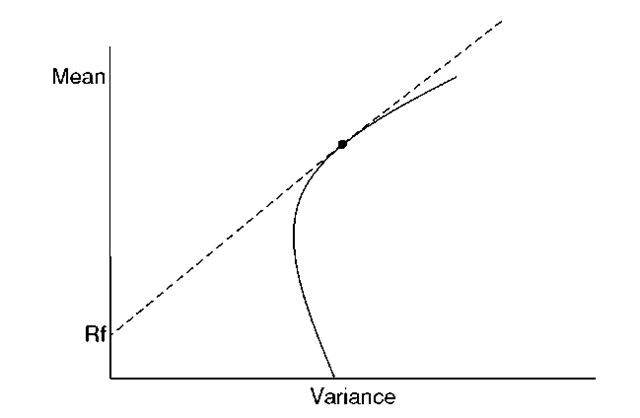
Thus, when there is a risk-free asset, all minimum-variance portfolios are a combination of a given risky asset portfolio with weights proportional to X* and the risk-free asset. This portfolio of risky assets is called the tangency portfolio because Xp* is independent of the level of expected return. If we draw the set of minimum-variance portfolios in the absence of a risk-free asset in a two-dimensional mean-standard deviation space like the curve GH in Figure 19.1, all efficient portfolios lie along the line from the risk-free asset through portfolio Xp*.
Sharpe (1964) proposes a measure of efficiency of a portfolio in terms of the excess return per unit risk. For any asset or portfolio with an expected return ma and standard deviation sa, the Sharpe ratio is defined as
Figure 19.1. Mean-Variance frontier with risk-free asset
The tangency portfolio Xp* is the portfolio with the maximum Sharpe ratio of all risky portfolios. Therefore, testing the mean-variance efficiency of a given portfolio is equivalent to testing if the Sharpe ratio of that portfolio is maximum of the set of Sharpe ratios of all possible portfolios.
Mean-Variance Efficiency and Asset Pricing Models
Capital Asset Pricing Models
The Markowitz mean-variance optimization framework is from the perspective of individual investor conditional on given expected excess returns and measure of risk of securities under consideration. The Capital Asset Pricing Model (CAPM) developed by Sharpe (1964) and Lintner (1965) asks what values of these mean returns will be required to clear the demand and supply if markets are efficient, all investors have identical information, and investors maximize the expected return and minimize volatility.
An investor maximizing the expected return and minimizing risk will choose portfolio weights for which the ratio of the marginal contribution to portfolio expected return to the marginal contribution to risk will be equal. In equilibrium, expected excess returns are assumed to be the same across investors. Therefore, suppose there exists a risk-free rate of interest, Rf, and let Zt = Ri-Rf be the excess return of the ith asset over the risk-free rate (Rf) then the expected excess return for the ith asset in equilibrium is equal to
where Zm is the excess return on the market portfolio of assets, Zm = Rm-Rf, with Rm being the return on the market portfolio.
In the absence of a risk-free asset, Black (1971) derived a more general version of the CAPM. In the Black version, the expected return of asset i in equilibrium is equal to the Black version, the expected return of asset i in equilibrium is equal to
where Rom is the return on the zero-beta portfolio associated with m. The zero-beta portfolio is described as the portfolio that has the minimum variance among all portfolios that are uncorrelated with m.
Closely related to the concept of trade-off between risk and expected return is the quantification of this trade-off. The CAPM or zero-beta CAPM provides a framework to quantify this relationship. The CAPM implies that the expected return of an asset must be linearly related to the covariance of its return with the return of the market portfolio and the market portfolio of risky assets is a mean-variance efficient portfolio. Therefore, studies ofmarket efficiency have been cast in the form of testing the Sharpe-Lintner CAPM and the zero-beta CAPM.
Under the assumption that returns are independently, identically (IID) multivariate normally distributed, empirical tests of the Sharpe-Lintner CAPM have focused on the implication of Equation (19.14) that the regression of excess return of the ith asset at time t, Zit = Rit-Rft on the market excess return at time t, Zmt = Rmt-Rft, has intercept equal to zero. In other words for the regression model
The null hypothesis of market portfolio being mean-variance efficient is:
Empirical tests of Black (1971) version of the CAPM model note that Equation (19.15) can be rewritten as
That is, the Black model restricts the asset-specific intercept of the (inflation adjusted) real-return market model to be equal to the expected zero-beta portfolio return times one minus the asset’s beta. Therefore, under the assumption that the real-return of N assets at time t, Rt = (Rit, …, RNt)0 is IID (independently identically distributed) multi-variate normal, the implication of the Black model is that the intercepts of the regression models
where the constant g denotes the expected return of zero-beta portfolio.
Arbitrage Pricing Theory
Although CAPM model has been the major framework for analyzing the cross-sectional variation in expected asset returns for many years, Gibbons (1982) could not find empirical support for the substantive content of the CAPM using stock returns from 1926 to 1975. His study was criticized by a number of authors from both the statistical methodological point of view and the empirical difficulty of estimating the unknown zero beta return (e.g. Britten-Jones, 1999; Campbell et al., 1997; Gibbons et al., 1989; Shanken, 1985; Stambaugh, 1982; Zhou, 1991). Ross (1977) notes that no correct and unambiguous test can be constructed because of our inability to observe the exact composition of the true market portfolio. Using arbitrage arguments, Ross (1977) proposes the Arbitrage Pricing Theory (APT) as a testable alternative. The advantage of the APT is that it allows for multiple risk factors. It also does not require the identification of the market portfolio.
Under the competitive market the APT assumes that the expected returns are functions of an unknown number of unspecified factors, say K (K < N):
where Rit is the return on asset i at time t, Ei is its expected return, fiik are the factor loadings, 8kt are independently distributed zero mean common factors and the eit are zero mean asset-specific disturbances, assumed to be uncorrelated with the 8kt.
As an approximation for expected return, the APT is impossible to reject because the number of factors, K, is unknown. One can always introduce additional factors to satisfy Equation (19.23). Under the additional assumption that market portfolios are well diversified and that factors are pervasive, Connor (1984) shows that it is possible to have exact factor pricing. Dybvig (1985) and Grinblatt and Titman (1987), relying on the concept of ”local mean-variance efficiency”, show that given a reasonable specification of the parameters of an economy, theoretical deviations from exact factor pricing are likely to be negligible. Thus, the factor portfolios estimated by the maximum likelihood factor analysis are locally efficient if and only if the APT holds (Roll and Ross, 1980, Dybvig and Ross, 1985).
Intertemporal Capital Asset Pricing Model (ICAPM)
The multifactor pricing models can alternatively be derived from an intertemporal equilibrium argument. The CAPM models are static models. They treat asset prices as being determined by the portfolio choices of investors who have preferences defined over wealth after one period. Implicitly, these models assume that investors consume all their wealth after one period. In the real world, investors consider many periods in making their portfolio decisions. Under the assumption that consumers maximize the expectation of a time-separable utility function and use financial assets to transfer wealth between different periods and states of the world and relying on the argument that consumers’ demand is matched by the exogenous supply, Merton (1973) shows that the efficient portfolio is a combination of one of mean-variance efficient portfolio with a hedging portfolio that reflects uncertainty about future consumption-investment state. Therefore, in Merton Intertemporal Capital Asset Pricing Model (ICAPM) it usually lets market portfolio serve as one factor and state variables serve as additional factors.
The CAPM implies that investors hold a mean-variance portfolio that is a tangency point between the straight line going through the risk-free return to the minimum-variance portfolios without risk-free asset in the mean-standard deviation space. Fama (1996) shows that similar results hold in multifactor efficient portfolios of ICAPM.
Estimation Errors and Portfolio Choice
The use of mean variance analysis in portfolio selection requires the knowledge of means, variances, and covariances of returns of all securities under consideration. However, they are unknown. Treating their estimates as if they were true parameters can lead to suboptimal portfolio choices (e.g. Frankfurther et al., 1971; Klein and Bawa, 1976; Jorion, 1986) have conducted experiments to show that because of the sampling error, portfolios selected according to the Markowitz criterion are no more efficient than an equally weighted portfolio. Chopra (1991), Michaud (1989), and others have also shown that mean-variance optimization tends to magnify the errors associated with the estimates.
Chopra and Zemba (1993) have examined the relative impact of estimation errors in means, variances, and covariances on the portfolio choice by a measure of percentage cash equivalent loss (CEL). For a typical portfolio allocation of large U.S. pension funds, the effects of CEL for errors in means are about 11 times as that of errors in variances and over 20 times as that of errors in covariances. The sensitivity of mean-variance efficient portfolios to changes in the means of individual assets was also investigated by Best and Grauer (1991) using a quadratic programming approach.
The main argument of these studies appears to be that in constructing an optimal portfolio, good estimates of expected returns are more important than good estimates of risk (covariance matrix). However, this contention is challenged by De Santis et al. (2003). They construct an example showing the estimates of Value at Risk (VaR), identified as the amount of capital that would be expected to be lost at least once in 100 months, using a $100 million portfolio invested in 18 developed equity markets to the sensitivity of different estimates of covariance matrix. Two different estimates of the covariance matrix of 18 developed equity markets are used -estimates using equally weighted 10 years of data and estimates giving more weights to more recent observations. They show that changes in estimated VaR can be between 7 and 21 percent.
The main features of financial data that should be taken into account in estimation as summarized by De Santis et al. (2003) are:
(i) Volatilities and correlations vary over time.
(ii) Given the time-varying nature of second moments, it is preferable to use data sampled at high frequency over a given period of time, rather than data sampled at low frequency over a longer period of time.
(iii) When working with data at relatively high frequencies, such as daily data, it is important to take into account the potential for autocorrelations in returns.
(iv) Daily returns appear to be generated by a distribution with heavier tails than the normal distribution. A mixture of normal distributions appear to approximate the data-generating process well.
(v) Bayesian statistical method can be a viable alternative to classical sampling approach in estimation (e.g. Jorion, 1986).


