Experimental Results
Databases
We used two databases in our face recognition across pose experiments, the CMU Pose, Illumination, and Expression (PIE) database [46] and the FERET database [39]. Each of these databases contains substantial pose variation. In the pose subset of the CMU PIE database (Fig. 8.4), the 68 subjects are imaged simultaneously under 13 poses totaling 884 images. In the FERET database, the subjects are imaged nonsimultaneously in nine poses. We used 200 subjects from the FERET pose subset, giving 1800 images in total. If not stated otherwise, we used half of the available subjects for training of the generic eigenspace (34 subjects for PIE, 100 subjects for FERET) and the remaining subjects for testing. In all experiments (if not stated otherwise), we retain a number of eigenvectors sufficient to explain 95% of the variance in the input data.
Fig. 8.4 Pose variation in the PIE database. The pose varies from full left profile (c34) to full frontal (c27) and to full right profile (c22). Approximate pose angles are shown below the camera numbers
Comparison with Other Algorithms
We compared our algorithm with eigenfaces [47] and FaceIt, the commercial face recognition system from Identix (formerly Visionics).1
We first performed a comparison using the PIE database. After randomly selecting the generic training data, we selected the gallery pose as one of the 13 PIE poses and the probe pose as any other of the remaining 12 PIE poses. For each disjoint pair of gallery and probe poses, we computed the average recognition rate over all subjects in the probe and gallery sets. The details of the results are shown in Fig. 8.5 and are summarized in Table 8.1.
In Fig. 8.5, we plotted 13 x 13 “confusion matrices” of the results. The row denotes the pose of the gallery, the column the pose of the probe, and the displayed intensity the average recognition rate. A lighter color denotes a higher recognition rate. (On the diagonals, the gallery and probe images are the same so all three algorithms obtain a 100% recognition rate.)
Eigen light-fields performed far better than the other algorithms, as witnessed by the lighter color of Fig. 8.5a, b compared to Fig. 8.5c, d. Note how eigen light-fields was far better able to generalize across wide variations in pose, and in particular to and from near-profile views.
Table 8.1 includes the average recognition rate computed over all disjoint gallery-probe poses. As can be seen, eigen light-fields outperformed both the standard eigenfaces algorithm and the commercial FaceIt system.
We next performed a similar comparison using the FERET database [39]. Just as with the PIE database, we selected the gallery pose as one of the nine FERET poses and the probe pose as any other of the remaining eight FERET poses. For each disjoint pair of gallery and probe poses, we computed the average recognition rate over all subjects in the probe and gallery sets, and then averaged the results. The results are similar to those for the PIE database and are summarized in Table 8.2. Again, eigen light-fields performed significantly better than either FaceIt or eigenfaces.
Fig. 8.5 Comparison with FaceIt and eigenfaces for face recognition across pose on the CMU PIE [46] database. For each pair of gallery and probe poses, we plotted the color-coded average recognition rate. The row denotes the pose of the gallery and the column the pose of the probe. The fact that the images in (a) and (b) are lighter in color than those in (c) and (d) implies that our algorithm performs better
Table 8.1 Comparison of eigen light-fields with FaceIt and eigenfaces for face recognition across pose on the CMU PIE database. The table contains the average recognition rate computed across all disjoint pairs of gallery and probe poses; it summarizes the average performance in Fig. 8.5
|
Algorithm |
Average recognition accuracy (%) |
|
Eigenfaces |
16.6 |
|
FaceIt |
24.3 |
|
Eigen light-fields |
|
|
Three-point norm |
52.5 |
|
Multipoint norm |
66.3 |
Table 8.2 Comparison of eigen light-fields with FaceIt and eigenfaces for face recognition across pose on the FERET database. The table contains the average recognition rate computed across all disjoint pairs of gallery and probe poses. Again, eigen light-fields outperforms both eigenfaces and Face It
|
Algorithm |
Average recognition accuracy (%) |
|
Eigenfaces |
39.4 |
|
FaceIt |
59.3 |
|
Eigen light-fields three-point normalization |
75.0 |
Overall, the performance improvement of eigen light-fields over the other two algorithms is more significant on the PIE database than on the FERET database. This is because the PIE database contains more variation in pose than the FERET database. For more evaluation results, see Gross et al. [23].
Bayesian Face Subregions
Owing to the complicated 3D nature of the face, differences exist in how the appearance of various face regions change for different face poses. If, for example, a head rotates from a frontal to a right profile position, the appearance of the mostly featureless cheek region only changes little (if we ignore the influence of illumination), while other regions such as the left eye disappear, and the nose looks vastly different. Our algorithm models the appearance changes of the different face regions in a probabilistic framework [28]. Using probability distributions for similarity values of face subregions; we compute the likelihood of probe and gallery images coming from the same subject. For training and testing of our algorithm we use the CMU PIE database [46].
Face Subregions and Feature Representation
Using the hand-marked locations of both eyes and the midpoint of the mouth, we warp the input face images into a common coordinate frame in which the landmark points are in a fixed location and crop the face region to a standard 128 x 128 pixel size. Each image I in the database is labeled with the identity i and pose φ of the face in the image:![]() As shown
As shown
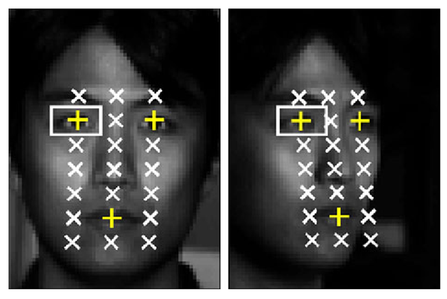
in Fig. 8.6, a 7 x 3 lattice is placed on the normalized faces, and 9 x 15 pixel subregions are extracted around every lattice point. The intensity values in each of the 21 subregions are normalized to have zero mean and unit variance.
As the similarity measure between subregions, we use SSD (sum of squared difference) values Sj between corresponding regions j for all image pairs. Because we compute the SSD after image normalization, it effectively contains the same information as normalized correlation.
Fig. 8.6 Face subregions for two poses of the CMU PIE database. Each face in the database is warped into a normalized coordinate frame using the hand-labeled locations of both eyes and the midpoint of the mouth. A 7 x 3 lattice is placed on the normalized face, and 9 x 15 pixel subregions are extracted around every lattice point, resulting in a total of 21 subregions
Modeling Local Appearance Change Across Pose
For probe image![tmp35b0-56_thumb[2] tmp35b0-56_thumb[2]](http://what-when-how.com/wp-content/uploads/2012/06/tmp35b056_thumb2_thumb.png) with unknown identity i, we compute the probability that Ii,p is coming from the same subject k as gallery image Ik,g for each face subregion
with unknown identity i, we compute the probability that Ii,p is coming from the same subject k as gallery image Ik,g for each face subregion![]() Using Bayes’ rule, we write:
Using Bayes’ rule, we write:
We assume the conditional probabilities![]()
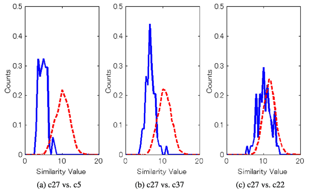
to be Gaussian distributed and learn the parameters from data. Figure 8.7 shows histograms of similarity values for the right eye region. The examples in Fig. 8.7 show that the discriminative power of the right eye region diminishes as the probe pose changes from almost frontal (Fig. 8.7a) to right profile (Fig. 8.7c).
It is reasonable to assume that the pose of each gallery image is known. However, because the pose φρ of the probe images is in general not known, we marginalize over it. We can then compute the conditional densities for similarity value sj as
and
If no other knowledge about the probe pose is given, the pose prior![]() is assumed to be uniformly distributed. Similar to the posterior probability defined in (8.5), we compute the probability of the unknown probe image coming from the
is assumed to be uniformly distributed. Similar to the posterior probability defined in (8.5), we compute the probability of the unknown probe image coming from the
Fig. 8.7 Histograms of similarity values Sj for the right eye region across multiple poses. The distribution of similarity values for identical gallery and probe subjects are shown with solid curves, the distributions for different gallery and probe subjects are shown with dashed curves
same subject (given similarity value Sj and gallery pose φΆ ) as
To decide on the most likely identity of an unknown probe image Iip = (i, φρ), we compute match probabilities between Iip and all gallery images for all face subregions using (8.5) or (8.6). We currently do not model dependencies between subregions, so we simply combine the different probabilities using the sum rule [29] and choose the identity of the gallery image with the highest score as the recognition result.
Experimental Results
We used half of the 68 subjects in the CMU PIE database for training of the models described in Sect. 8.3.2. The remaining 34 subjects are used for testing. The images of all 68 subjects are used in the gallery. We compare our algorithm to eigenfaces [47] and the commercial FaceIt system.
Experiment 1: Unknown Probe Pose
For the first experiment, we assume the pose of the probe images to be unknown. We therefore must use (8.6) to compute the posterior probability that probe and gallery images come from the same subject. We assume![tmp35b0-70_thumb[2] tmp35b0-70_thumb[2]](http://what-when-how.com/wp-content/uploads/2012/06/tmp35b070_thumb2_thumb.png) to be uniformly distributed, that is,
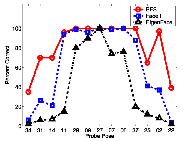
to be uniformly distributed, that is,![tmp35b0-71_thumb[2] tmp35b0-71_thumb[2]](http://what-when-how.com/wp-content/uploads/2012/06/tmp35b071_thumb2_thumb.png) Figure 8.8 compares the recognition accuracies of our algorithm with eigenfaces and FaceIt for frontal gallery images. Our system clearly outperforms both eigenfaces and FaceIt. Our algorithm shows good performance up until 45° head rotation between probe and gallery image (poses 02 and 31). The performance of eigenfaces and FaceIt already drops at 15° and 30° rotation, respectively.
Figure 8.8 compares the recognition accuracies of our algorithm with eigenfaces and FaceIt for frontal gallery images. Our system clearly outperforms both eigenfaces and FaceIt. Our algorithm shows good performance up until 45° head rotation between probe and gallery image (poses 02 and 31). The performance of eigenfaces and FaceIt already drops at 15° and 30° rotation, respectively.
Fig. 8.8 Recognition accuracies for our algorithm (labeled BFS), eigenfaces, and Face It for frontal gallery images and unknown probe poses. Our algorithm clearly outperforms both eigenfaces and Face It
Experiment 2: Known Probe Pose
In the case of known probe pose, we can use (8.5) to compute the probability that probe and gallery images come from the same subject. Figure 8.9 compares the recognition accuracies of our algorithm for frontal gallery images for known and unknown probe poses. Only small differences in performances are visible.
Figure 8.10 shows recognition accuracies for all three algorithms for all possible combinations of gallery and probe poses. The area around the diagonal in which good performance is achieved is much wider for our algorithm than for either eigen-faces or Face It. We therefore conclude that our algorithm generalizes much better across pose than either eigenfaces or Face It.

![Comparison with FaceIt and eigenfaces for face recognition across pose on the CMU PIE [46] database. For each pair of gallery and probe poses, we plotted the color-coded average recognition rate. The row denotes the pose of the gallery and the column the pose of the probe. The fact that the images in (a) and (b) are lighter in color than those in (c) and (d) implies that our algorithm performs better Comparison with FaceIt and eigenfaces for face recognition across pose on the CMU PIE [46] database. For each pair of gallery and probe poses, we plotted the color-coded average recognition rate. The row denotes the pose of the gallery and the column the pose of the probe. The fact that the images in (a) and (b) are lighter in color than those in (c) and (d) implies that our algorithm performs better](http://what-when-how.com/wp-content/uploads/2012/06/tmp35b052_thumb.png)

![tmp35b0-60_thumb[2] tmp35b0-60_thumb[2]](http://what-when-how.com/wp-content/uploads/2012/06/tmp35b060_thumb2_thumb.png)
![tmp35b0-63_thumb[2] tmp35b0-63_thumb[2]](http://what-when-how.com/wp-content/uploads/2012/06/tmp35b063_thumb2_thumb.png)
![tmp35b0-64_thumb[2] tmp35b0-64_thumb[2]](http://what-when-how.com/wp-content/uploads/2012/06/tmp35b064_thumb2_thumb.png)

![tmp35b0-68_thumb[2] tmp35b0-68_thumb[2]](http://what-when-how.com/wp-content/uploads/2012/06/tmp35b068_thumb2_thumb.png)

