Symbol-Table-Handling Techniques (Compiler Writing) Part 2

Ordered Symbol Tables

In this and the following two subsections, we describe symbol-table organizations in which the table position of a variable’s set of attributes is based on the variable’s name. In such circumstances, an insertion must be accompanied by a lookup procedure which determines where in the symbol table the variable’s attributes should be placed. The actual insertion of a new set of attributes may generate some additional overhead primarily because other sets of attributes may have to be moved in order to achieve the insertion. These notions will be illustrated often in the remaining discussion in this section.

An ordered symbol table is illustrated in Fig. 8-7. Note that the table is lexically ordered on the variable names. While a number of table-lookup strategies can be applied to such a table organization, we will examine the two most popular search techniques: the linear search and the binary search.

In the previous subsection we discussed the linear search with respect to an unordered symbol-table organization. The question that must be addressed is whether ordering the table is beneficial when using the linear-search technique. The lookup operation still requires an average search length of (n + l)/2 if the search argument is in the table. An analysis deriving this result is identical to that given in the previous subsection for unordered tables. Note, however, that if the search argument is not in an ordered table, its absence can be detected without having to search the complete table. Upon encountering the first argument in the table which is lexically greater than the search argument, it is decidable that the search argument is not in the table. Therefore, the average length of search required to determine if an argument is in an ordered table.or not is (n + l)/2 (again, assuming the same analysis given previously).

Using an ordered table organization avoids the necessity of a complete table search. An additional complexity, however, is introduced when performing the insertion operation. For example, if the variable COUNT is inserted in the table which is stored sequentially as shown in Fig. 8-7, then the elements lexically larger than COUNT must be moved down in the table to make room for the insertion of the set of attributes for COUNT. Therefore, using a linear-search technique on an ordered table, an insertion operation requires n — c comparisons followed by c moves (i.e., a total of n basic operations). The movement of a table record can be eliminated by using a singly linked list form of table representation which facilitates a single-step insertion. This approach, however, requires that an additional link field be attached to each table record.

From the previous analysis, we can conclude that ordering the symbol table affords few appreciable advantages over the unordered organization if a linear search is used.

Variable Name	Type	Dimension	Other Attributes
ANS	1	0
B	1	0
COMPANY*	2	1
FIRST	1	0
FORM1	3	2
M	6	0
X3	1	0

Figure 8-7 An ordered symbol table.

In fact the one major advantage is that the ordered symbol table can be used in the direct generation of a cross-reference listing, whereas an unordered table would have to be sorted before printing such a listing.

It can be shown that the most efficient way to search an ordered table using only comparisons is the binary search (see Knuth, 1973). In this search strategy we begin by comparing a search argument, say X, with the middle element of the table. This comparison either locates the desired element or dictates which half of the table should be searched next. If the desired element is not located, the appropriate half of the table is selected as a new subtable upon which the halving or bisection procedure is repeated. The middle element of the new subtable is compared with the search element as before, and this process is continued until the desired table element is found. For example, a search for the variable named FORM1 in the table given in Fig. 8-7 produces the following sequence of probes: FIRST, M, and finally FORM1.

The following algorithm formally describes the binary search method.

Function BINARY_SEARCH(SARG). Given a table of global records R1, R2…..Rn whose variable names as denoted by NAME, are in increasing order, this function searches the structure for a given search argument SARG. The local variables B and E denote the lower and upper limits of the search interval, respectively. If any NAME, matches SARG, the index i is returned. If no match is found, the negation of the latest value of i is returned.

The size of the set of table records that are potentially accessible in a particular iteration (i.e., step 2 in Function BINARY_SEARCH) grows as the square of the iteration. That is, in the first pass one record is compared, in the second pass two records are potential candidates for comparison, in the third pass four records are potential candidates, and in general, in the nth pass 2"~ records are potential candidates. From this analysis, it is easy to establish that the maximum length of search using a binary search is [log2«J + 1 for a table of size n. Therefore, in the example table given in Fig. 8-7, the maximum length of search is [log27j + 1 or 3.

The average length of search is given in the following expression:

(a) PL/I

(b) C

Table size n

Running time, seconds

Table size n

Running time, seconds

Linear

Binary

Linear

Binary

7

10.34

12.79

1

8.5

9.5

15

27.53

30.33

15

•26.8

24.3

31

87.49

70.25

31

89.3

57.7

While a binary search may improve the table-lookup operation, the problem ~ of inserting an element into an ordered table persists. Recall that in Function BINARY_SEARCH a negative index is returned if the search element is not found. The absolute value of this index generally points to the lexically largest variable name which is less than the search argument. (Some exceptions to this rule occur, for example, when the search argument is less than any element in the table, in which case a -1 is returned.) Therefore Function BINARY_SEARCH yields the position at which the new record should be inserted. Unfortunately, on the average (n + l)/2 moves are still required to insert the record.

Tree-Structured Symbol Tables

The time to perform a table-insertion operation can be reduced from that of an ordered table by using a tree-structured type of storage organization. In this type of organization an attempt is made to reflect the search structure of the binary search in the structural links of a binary-search tree.

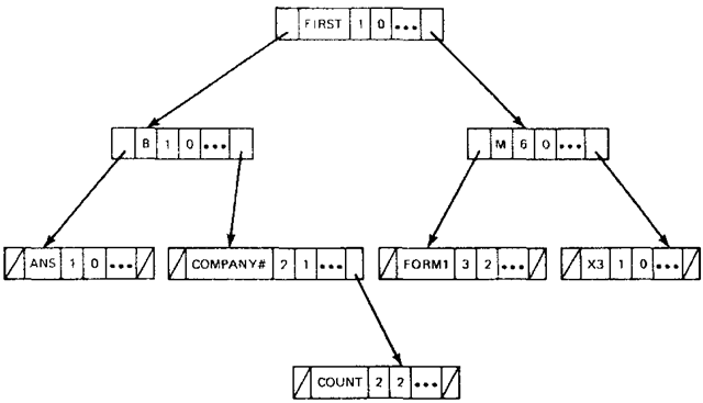
A binary tree-structured symbol table that contains the same records as the table in Fig. 8-7 is illustrated in Fig. 8-8a. Note that two new fields are present in a record structure. These two link fields will be called the left pointer and right pointer fields. Access to the tree is gained through the root node (i.e., the top node of the tree). A search proceeds down the structural links of the tree until the desired node is found or a NULL link field (denoted by /) is encountered. In the latter case, the search is unsuccessful, since a match between the search argument and the names in the table is not achieved.

The tree representation given in Fig. 8-8a shows only the logical relationship between table records in the tree. Because link fields define only the logical relationships between the table records, we are free to store the records in a contiguous area and in any order, provided the correct structural relationships between nodes are preserved. Figure 8-8b depicts the more familiar representation for a table (i.e., a representation in which table records are physically adjacent). In the figure, the pointer-field value of zero represents a NULL structural link. In this representation the root node is always located at the first record location in the table.

In a binary-tree organization, a new record is inserted as a leaf node (i.e., a node with NULL in both link fields) in a tree. This insertion is completed so as to preserve a lexical ordering of table records as dictated by the structural links of the tree. To describe the notion of lexical ordering more clearly, the concepts of a left and right subtree must be introduced.

The left subtree of a node X is defined to be that part of the tree containing all those nodes reachable from the left branch of X. For example, the set of nodes for the variables B, ANS, and COMPANY* plus the interconnecting structural links form the left subtree of the node for the variable FIRST in Fig. 8-8.

 

Table Position	Name Field	Type	Dimension	Other Attributes	Left Pointer	Right Pointer
1	FIRST	1	0		....... !' 2	5
2	B	1	0		3	4
3	ANS	1	0		0	0
4	COMPANY #	2	1		0	0
5	M	6	0		6	7
6	F0RM1	3	2		0	0
7	X3	1	0		0	0
			(6)

Figure 8-8 Binary-tree organization of a symbol table showing (a) the logical relationships and (b) a physical representation.

The right subtree has an obvious complementary meaning.

Therefore, in a binary-tree organization, the tree is ordered such that every node in its left subtree precedes lexicographically the root node of the tree. Similarly, every node in its right subtree follows lexicographically the root node of the tree. This ordering holds for all subtrees in a tree as well. For example, if a record for the variable COUNT is inserted in the tree given in Fig. 8-8a, it is treated as a leaf node and is placed to the right of the record for the variable COMPANY*. The insertion is shown in Fig. 8-9.

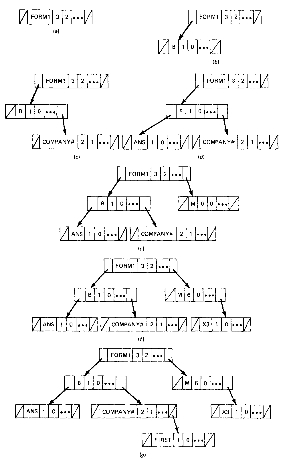
It is important to realize that because of this insertion strategy the organization of the tree structure is dependent upon the order of insertion. To illustrate this point, let us examine Fig. 8-8a.

Figure 8-9 The insertion of a record for the viable name COUNT

This tree structure is created if, for example, the records are inserted in the order

Figure 8-10 shows the stages in the development of the tree assuming the latter insertion order.

Because records are inserted so as to preserve a particular ordering, an insertion operation must always include the same tree-search procedure required for a lookup operation. This combined search procedure is described in Function BIN_TREE, which follows. In the algorithm we distinguish between the insertion and lookup operations by a logical parameter INSERT. If INSERT is true, an insertion operation is requested; if it is false, a lookup operation is implied. For both operations, SARG is a parameter containing the search argument, i.e., the name of the variable being inserted or searched for. DATA is a parameter containing additional attribute information for an insertion operation.

If the operation is an insertion and it is successful, the location of the new node is returned. If it is unsuccessful, a negated pointer value is returned which indicates the position of a previously inserted record with the same name as the search argument.

Figure 8-10 The construction of a tree-structured symbol table

For a table-lookup operation, a successful search returns the location of the record with a name field that matches the search argument. If the search is unsuccessful (i.e., the variable has not been previously declared), then a negated pointer value is returned, indicating the last node examined during the search. This value can be used to insert a new node as part of an error-recovery procedure.

Function BIN_TREE(INSERT, SARG, DATA, ROOT). Given the parameters INSERT, SARG, and DATA as described previously, as well as ROOT, which is a variable containing the location of the root node in the tree, this function performs the requested operation on the tree-structured symbol table. The global record node, NODE, has a name field called NAME, the attribute fields of a record node are denoted by ATTR, and the left pointer and right pointer fields in a record node are identified by LPTR and RPTR, respectively. T and P are temporary pointer variables. If the requested operation is performed successfully, the address of any newly created node is returned; otherwise, the negation of the latest value of T is returned.

 

 

 

 

The algorithm should be easy to understand based on the previous discussion. Basically a search proceeds down the tree structure via a series of comparisons which are performed iteratively in step 3 of the algorithm. If a match occurs, then either a negated pointer value is returned, indicating an error in the insertion operation, or the position of the record with the name equal to the search argument is returned for a lookup operation.

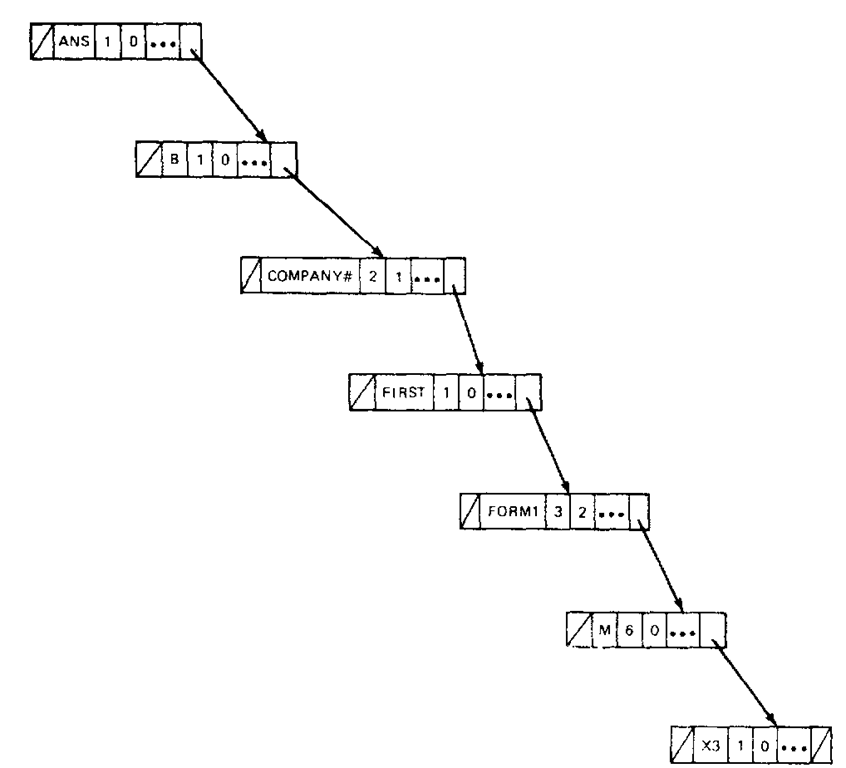
Figure 8-11 The ordered insertion of a sample set of variables

If a match is not found, that is, a NULL link field is encountered in step 3, then either a negated pointer value is returned for the lookup operation or a new record is created and appended to the tree in an insertion operation.

A major problem exists with the binary tree organization just described. Since insertion always takes place at the leaves of the tree, a search tree can become very unbalanced. For example, it is a common practice when writing large programs to declare the variables in a module in lexicographic order. If this practice is applied to a module containing the variables in Fig 8-8, a tree as depicted in Fig. 8-11 will be created. It is obvious that in this situation the binary tree structure has degenerated to an ordered linked list with an average search length of (n -t- l)/2. Hibbard (1962) showed that for randomly generated trees an average search length of 1.4 log2n is expected.

The ideal search tree is, of course, one in which all maximum-length search paths are of equal or nearly equal length and thus elongated search paths such as the one shown in Fig. 8-11 are avoided. This ideal situation is realized in a tree-structured organization called an optimally balanced binary tree. In such a structure the distances (i.e., path length) from the root node to any two incomplete nodes of the tree differ by at most 1. By an incomplete node, we mean a node in which at least one of its link fields has a NULL value. Note that our definition of an optimally balanced tree is somewhat restrictive in the sense that all nodes are considered to have the same probability of access. For a more general definition, see Knuth (1973).

The search trees in Figs. 8-8 and 8-9 are both optimally balanced. Unfortunately, it is difficult to keep a tree structure optimally balanced when records are continually inserted into the structure. Consider the optimally balanced tree given in Fig. 8-12. The insertion of a record for the variable ANS constitutes almost a complete reorganization (i.e., a change in every link field) of the tree structure to arrive at an optimally balanced tree such as that in Fig. 8-8.

Figure 8-12 Example of optimal balanced tree where the insertion of ANS requires a complete reorganization

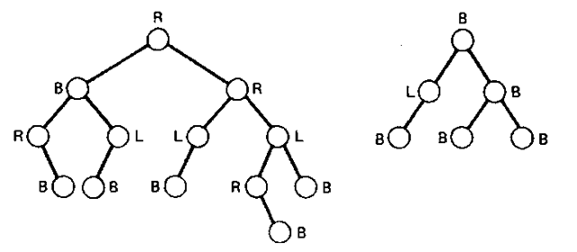
Figure 8-13 Examples of AVL trees.

Therefore, to attain an optimally balanced tree may require at least the examination of every node in the tree. Such an examination takes on the order of n basic operations.

By reducing the balancing criteria from optimally balanced to almost optimally balanced as defined by Adel’son-Vel’skii and Landis (1962), we are able to locate, to insert, or to delete an item in the order of log2« basic operations. An A VL tree (named after the original authors) is a binary-search tree in which each node of the tree is in one of three states:

1. A node is left-heavy if the longest path in its left subtree is one longer than the longest path of its right subtree.

2. A node is balanced if the longest paths in both of its subtrees are equal.

3. A node is right-heavy if the longest path in its right subtree is one longer than the longest path in its left subtree.

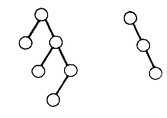
If each node in the tree is in one of the three previous states, the tree is said to be balanced; otherwise it is unbalanced. Each node in the tree structure contains a balance indicator field which indicates the current state of node. Figure 8-13 illustrates two balanced trees with the state, left (L), balanced (B), or right (R), marked on each node. Figure 8-14 represents examples of unbalanced trees.

Let us now examine the symbol-table operations of insertion and lookup as they apply to AVL trees. Again a lexicographic ordering is assumed in the relationships between record nodes of the tree-symbol table and, therefore, node insertion must be preceded by a search procedure to locate where the node should reside.

Figure 8-14 Examples of unbalanced trees.

A placement of the node using the strategy in Function BIN_TREE can cause the AVL tree to become Unbalanced. Upon detection of an unbalanced tree, a rebalancing strategy must be applied. We next concentrate on how to detect an unbalanced tree and how to rebalance such a tree.

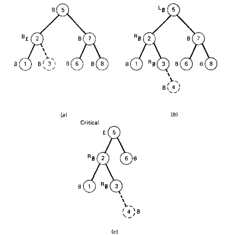
In the following discussion, it is assumed that a new node is inserted at the leaf level (as either a left or a right subtree of some incomplete node). The only nodes which can have their balance indicator changed by such an insertion are those which lie on a path between the root of the tree and the newly inserted leaf. The possible changes which can occur to a node on this path are as follows:

1. The node was either left- or right-heavy and has now become balanced.

2. The node was balanced and has now become left- or right-heavy.

3. The node was heavy and the new node has been inserted in the heavy subtree.

If condition 1 applies to a current node, then the balance indicators of all ancestor nodes of this node remain unchanged, since the longest path in the subtree (of which the current node is its root) remains unchanged. When condition 2 applies to a current node, the balance indicators of the ancestors of this node will change. If condition 3 applies to a current node, the tree has become unbalanced and this node has become critical. Figure 8-15 contains examples of the three cases which can arise. The dotted branch and node denote the new element which is being inserted.

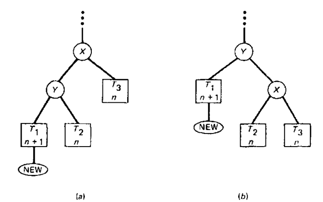
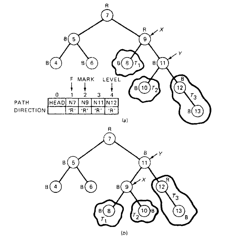
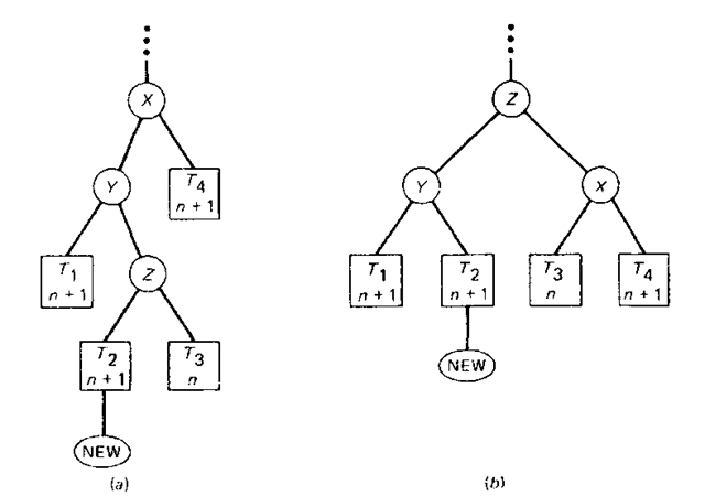
Let us now address the problem of rebalancing a tree when a critical node is encountered. There are two broad cases which can arise, each of which can be further subdivided into two similar subcases. A general representation of case 1, which is often called single rotation, is given in Fig. 8-16. The rectangles labeled 7\, T2, and T3 represent subtrees and the node labeled NEW denotes the node being inserted. The expression at the bottom of each rectangle denotes the maximum path length in that subtree after insertion. With the insertion of node NEW in Fig. 8-16o the node X becomes critical since the maximum path lengths for the left subtree and the right subtree are n + 2 and n, respectively. To rebalance, we simply rotate the positions of X and Y as shown to arrive at a balanced tree. A specific example of the second subcase for single rotation (i.e . X is critically unbalanced to the right) is exemplified in Fig. 8-17. The PATH and DIRECTION vectors are explained in the Function AVL_TREE which follows.

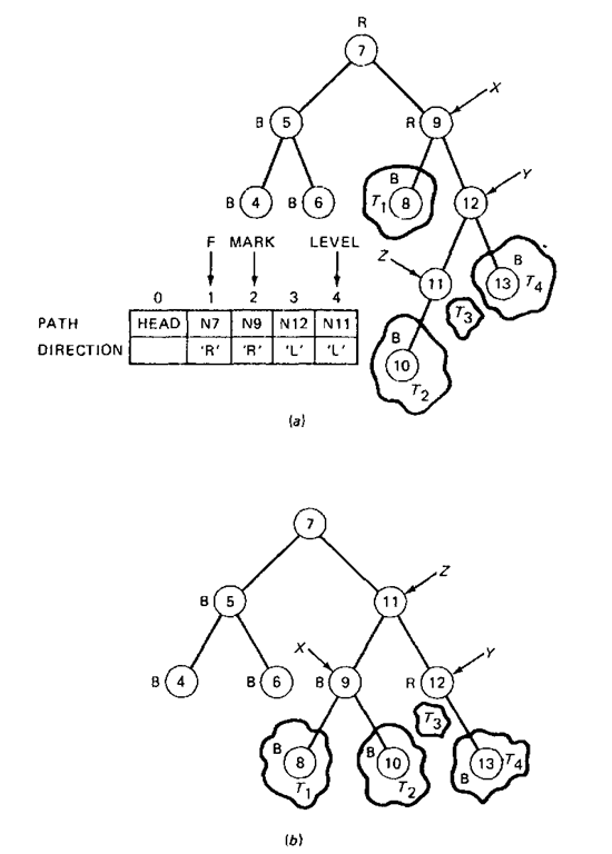
The second case, called double rotation, is illustrated in Fig. 8-18. It is much like the first, except that node Y becomes heavy in an opposite direction to that in which X was heavy. It is necessary to move node Z up the tree in such a way as to reduce the maximum path length of the left subtree of X. In effect, two interchanges are required: one between Y and Z, and then one between Z and X. Again, a specific example of the second subcase (i.e., X is critically unbalanced to the right) is shown in Fig. 8-19.

We now consider the formulation of Function AVL_TREE for the insertion and lookup of a search argument SARG. The record structure (NODE) for the tree consists of a left pointer field (LPTR), a name field (NAME), a set of attribute fields (ATTR), a balance indicator (Bl), and a right pointer field (RPTR).

Figure 8-15 Examples of insertions into a balanced tree, (a) Condition 1. (b) Condition 2 (<) Condition 3.

Figure 8-16 Rebalancing using a single rotation.

Figure 8-17 Example of single rotation, (a) Before balancing (h) After balancing

Figure 8-18 Rebalancing using a double rotation

Figure 8-19 Example of double rotation, (a) Before balancing. (/>) After balancing.

The balance indicator can have values of ‘L’ (left-heavy), ‘R’ (right-heavy), or ‘B’ (balanced). The root node is pointed to by the left pointer of a special node called the list head. The list-head node is important in the following algorithm because it ensures that the algorithm is general enough to handle rotations involving the root node of the tree. The list head is accessible through the pointer variable HEAD, and its balance indicator Bl always has a value of ‘L’. The logical variable INSERT and the variables SARG and DATA assume the same roles as in Function BIN_TREE.

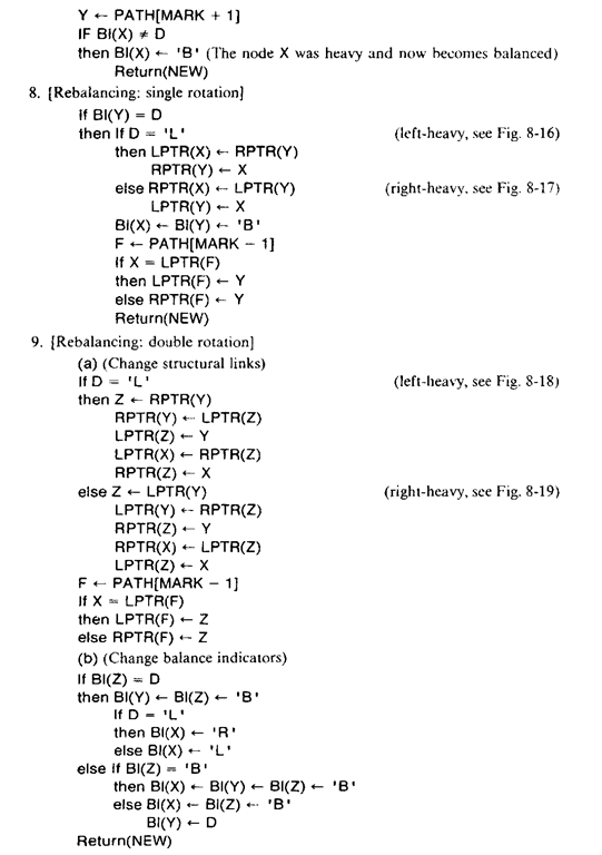
Function AVL_TREE(INSERT, SARG, DATA, HEAD). Given a tree representation as just discussed and the parameters INSERT, SARG, DATA, and HEAD, this function performs the table lookup and insertion operations on an AVL tree. The array PATH is used to store the addresses of the nodes between the list head and the point in the tree where the insertion is made. The corresponding vector DIRECTION is used to store the direction of each branch in this path. The values of ‘L’ and ‘R’ are used to denote a left and right branch, respectively. The variable MARK denotes the index of an array element in PATH which contains the address of the critical node (X). F points to the parent of the critical node before rebalancing takes place. The variables X, Y, and Z are pointer variables whose functions have been previously described. LEVEL is an index variable. NEW is the address of the new node created, and this address is returned if the requested operation is successful. Otherwise, either NULL or the negation of the address of T is returned. T is a temporary pointer used in traversing the tree from the root to where the node is to be being inserted.

 

 

 

 

 

 

 

 

 

Steps 1 through 4 are closely patterned after Function BIN_TREE. If an insertion operation is performed, step 4 attaches the new node to the existing tree. In addition, it stores into vectors PATH and DIRECTION the address of the nodes on the path between the root node and the leaf being inserted, and direction of the path at each node, respectively. If a NULL link field is encountered in step 4 during a lookup operation, a negated pointer value of the current node T is returned, thereby signaling an error condition. Step 5 of the algorithm searches for an unbalanced node which is closest to the new node just inserted. In step 6 the balance indicators of the nodes between the unbalanced node found in the previous step and the new node are adjusted. Step 7 determines whether or not there is a critical node. If there is, control proceeds either to step 8 (single-rotation) or step 9 (double-rotation). When no critical node is found, the balance indicator of the unbalanced node found in step 5 is adjusted. The last two steps of the algorithm correspond to case 1 and case 2 in the previous discussion, and rebalancing of the tree is performed in each case. The reader should trace through the algorithm for the examples given in Figs. 8-17 and 8-19.

Let us look more closely at the performance of Function AVI__TREE. It can be shown that the maximum path length m in an AVL tree of n nodes is 1.5 log2(« + 1) (see Stone, 1972). Knuth (1973) shows with the aid of some empirical evidence that the expected search time is log2(« + 1) + a constant. Therefore, for a reasonable size n, the AVL tree organization is almost as good as an optimally balanced tree organization.

A number of other suboptimal search-tree organizations have been proposed, and a survey of these methods can be found in Knuth (1973) and Nievergelt (1974). Two of the more popular organizations are the weight-balanced (WB) tree (Knuth, 1973; Baer, 1975) and the bounded-balance (BB) tree (Nievergelt and Reingold, 1973). In a weight-balanced tree certain access frequencies are assumed to be known for the table elements. In particular letdenote the access frequencies of the variableswhereand

denote the frequencies with which search arguments would lie between the variable names (i.e., a, is the frequency with which a search argument S satisfiesThen the average length of search for both successful and unsuccessful searches is

where /, is the level of a node or the level at which it is discovered that the search argument is not in the table. An optimal weight-balanced tree is one in which expression (2) is minimized.

Two major problems exist with weight-balanced trees. The most obvious is that the sets of frequenciesare never really known a priori during the compilation process. Second, the time to construct such trees is on the order of «3 basic operations.

BB trees are based on a height-balancing principle as are AVL trees. The difference is that the balancing parameter attempts to provide a compromise between short search time and infrequent rebalancing in the following sense. A tree T is of bounded balance a, or is BB[a], if and only if, for each subtree T’ of r, the fraction of nodes in the left subtree of T lies between a and 1 – a. Therefore, in a tree of bounded balance 1 /4, one subtree of a node may be up to 3 times the size of the other. The rebalancing of a bounded-balanced tree has been shown to be slightly less time-consuming than for AVL trees.

Baer and Schwab (1977) have conducted a comparative study of these different search-tree organizations. The results of their study showed that "the AVL tree construction is the most efficient when the operations on trees are limited to insertion and queries." Some of the other search-tree organizations may provide better performance for large directories in file-processing applications; however, the AVL tree appears to be the best search-tree organization for a symbol table.

Before we conclude our discussion of binary tree-structured symbol tables, we should mention some other tree-oriented organizations. In particular, a forest of six trees has been used in the FORTRAN H compiler (IBM). A separate tree is constructed for identifiers of lengths 1 through 6. The FORTRAN H compiler also uses tree-structured tables for constants and statement numbers.

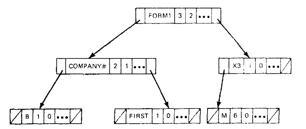
Severance (1974) has suggested that in situations in which a large number of variables appear in a symbol table, a special w-ary type of tree structure called a trie be used in conjunction with a binary tree. The basic idea is to use a trie node with 26 link fields (one for each letter in the alphabet) at the first level and to use a binary tree structure at lower levels of the structure. Figure 8-20 exhibits an example of this type of organization.

Figure 8-20 A trie-tree symbol-table organization.