Two-Dimensional Active Contours (Snakes) Part 2 (Biomedical Image Analysis)

Gradient Vector Flow

In the context of the greedy snake algorithm, multilevel blurring was mentioned as one method to increase the capture range of the snake. Another powerful method to increase the capture range and to provide an external force field that stabilizes the behavior of the snake is to diffuse the edge image. Xu and Prince35 propose a gradient vector flow field, computed from the edge image through

where u and v are the forces in the x and y directions, respectively, f is the edge image, obtained, for example, by applying the Sobel operator, and ^ is a normalization factor that determines the amount of smoothing. Equation (6.30) can be discretized by using the convolution-based discrete Laplacian operator.

The gradient fieldscan be computed outside the iteration loop. The gradient vector flow field can be computed before the application of the snake algorithm and used directly for the forces fx and fy in Equation (6.29). Assume that two convolution-based operators, acting on an image I(x,y), Laplace(I) and Sobel(I), are available. A variant, NSobel(I), computes the edge image but ensures that all values are normalized to lie in the range 0 to 1. Furthermore, the directional differences diff_x (I) and diff.y (I) are defined as pointwise central differences

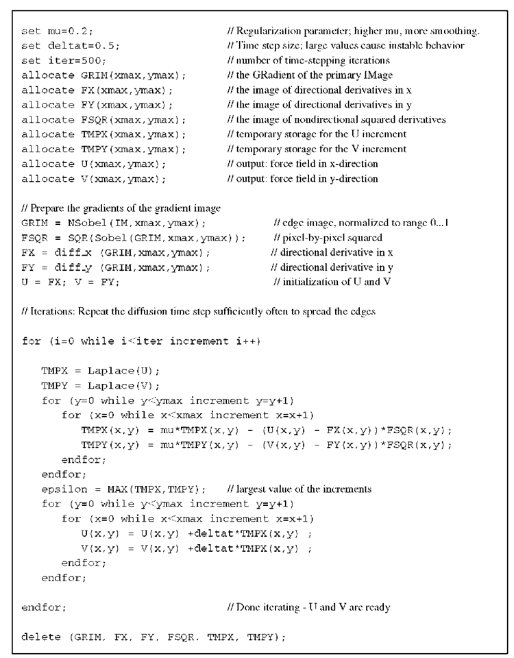
With these prerequisites, the gradient vector flow can be computed using Algorithm 6.2.

Algorithm 6.2 shows slow convergence, and a large number of iterations need to be performed to provide a reasonable spread of the edges. More efficient implementations are possible, primarily by using multigrid techniques. On a 256 x 256 image, Algorithm 6.2 takes on the order of tens of seconds to converge. Even with an efficient implementation, several seconds of computation time are required. Numerical stability depends critically on the selection of a small enough A t, which in turn depends on If the grid space is assumed to be unity, A t should be smaller than 1/4^.35 In practical applications, even smaller values were necessary to prevent diverging behavior, and the conditionwas determined experimentally. Therefore, A t should be selected to be a safe margin less than in the rangeConvergence can easily be monitored by displaying € over the progression of the time-stepping loop. Furthermore, it is critically important that the edge image be normalized to the value range of 0 to 1; otherwise, the algorithm will not converge.

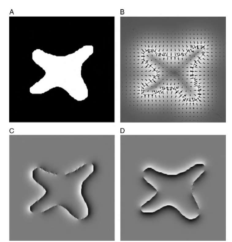
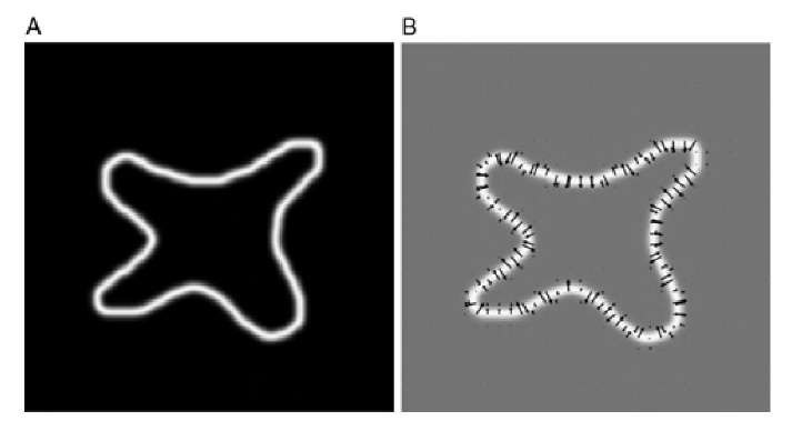
Figures 6.8 and 6.9 demonstrate the superior capture range of the gradient vector field compared with a blurred edge image. It can be seen in Figure 6.8B that almost the entire interior of the feature has nonzero forces, whereas the interior of a conventional blurred edge image [Equation (6.5)] does not exhibit any forces in most of the interior space (Figure 6.9B). This behavior has two consequences. In a regular gradient image, the snake is placed outside the feature and shrinks until it locks onto the edge. When andfirst-order central differences to obtain df/dx and df/dy, and the squared result of the Sobel operator applied on f to obtainBy using a first-order Euler approximation, u and v can be computed iteratively with a time step

Algorithm 6.2 Gradient vector flow. This algorithm computes the gradient vector flow field of an input image. The input image is IM(x,y) and is subjected to the Sobel operator immediately to obtain the edge image. From the edge image, the directional and nondirectional gradients FX, FY, and FSQR are computed. A temporary image per direction is needed to hold the Laplacian images (TMPX and TMPY). The output of the algorithm are the forces U and V. Instead of stepping through the specified number of iterations, the variable epsilon may be used as a criterion of convergence and iteration stopped once epsilon drops below a predetermined threshold.

FIGURE 6.8 Gradient vector flow used as the external image force for snakes. In part A, a simple image feature with concave regions is presented. Part B shows the magnitude of the gradient vector flow field with the forces superimposed as small arrows. Parts C and D are gray-scale representations of the forces acting in the x and y directions, respectively (U and V in Algorithm 6.2), where medium gray represents no force, dark shades represent forces in the negative direction (left and up, respectively), and light shades represent forces in the positive direction (right and down, respectively).

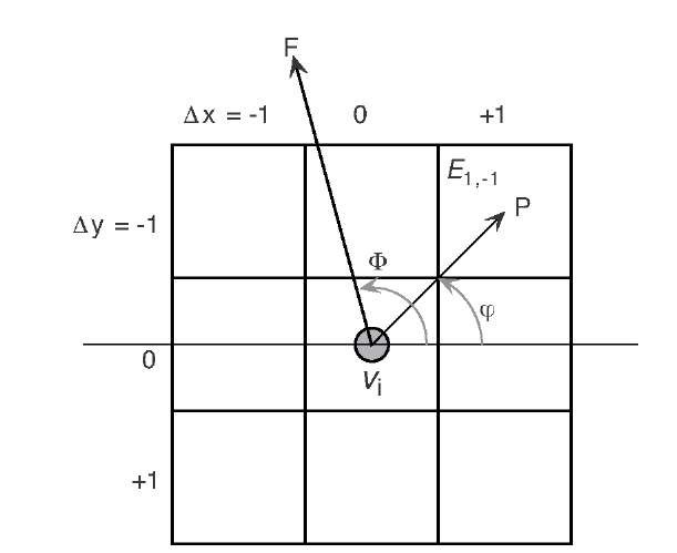
Although gradient vector flow is most commonly used in conjunction with the force formulation, it is possible to implement gradient vector flow forces in a greedy algorithm as well. In this case, the force vectors can be used to fill an n x n neighborhood with energy values that represent the external energy in the greedy search algorithm (Figure 6.10). The gradient vector flow imposes a force F on vertex vi of the snake. Each of the eight neighborhood pixels is connected to the vertex through a pixel vector p.

FIGURE 6.9 Conventional computation of the gradient field for the snake algorithm using Equation (6.5). (A) shows the edge image of Figure 6.8A, blurred twice by a Gaussian kernel with a = 1.6 and a 11 x 11 neighborhood. In (B), the gradient forces are shown by magnitude (gray shade) and in vector form (arrows). The capture range (i.e., the area surrounding the edge in which the forces are nonzero) is considerably smaller than the gradient vector flow forces in Figure 6.8B.

The corresponding energy at the pixel with displacement A x and A y can therefore be computed through

where the index k covers all eight neighbor pixels, and the displacement (A x,A y) that minimizes the energy of the vertex in its neighborhood is chosen.

FIGURE 6.10 The search neighborhood of a greedy snake vertex can be filled with energy values based on gradient vector flow by multiplying the force vector F by the potential pixel displacement vector p.

Topologically Adaptive Snakes

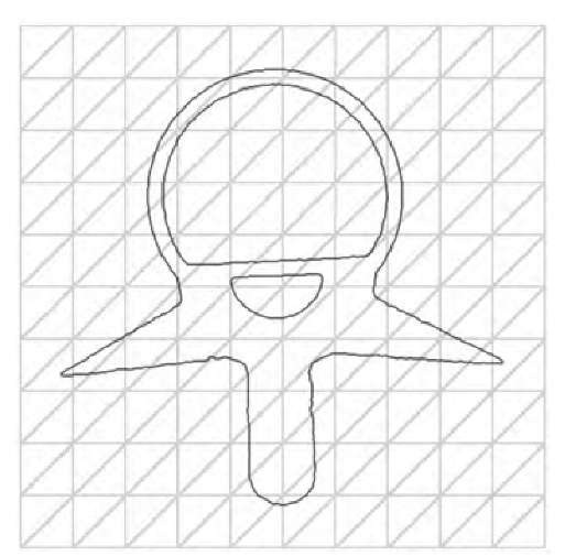
An extension of the snake model was presented by McInerney and Terzopoulos.21 Up to this point, snakes were assumed to be the topological equivalent of a circle. This restrictive assumption can be overcome if a snake is allowed to split or if two intersecting snakes are allowed to merge. McInerney and Terzopoulos propose projecting the snake onto a simplicial cell decomposition of the image surface. In two-dimensional space, this decomposition can be realized by subdividing the plane into equal squares, then subdividing each square into two triangles (Freudenthal triangularization), as shown in Figure 6.11. In the presence of a single snake, each triangle will therefore be either inside or outside the snake, or it will intersect the snake. Triangles that intersect the snake can be thought of as boundary cells, and the boundary cells approximate the snake contour. By using cells as a shape approximation, a snake can either be found to be self-intersecting or two snakes can be found to share a series of consecutive cells. In these cases, the single snake is split or the two snakes are merged, respectively. This process implies that the snake implementation needs the ability to handle multiple snakes and to allocate and delete snakes dynamically.

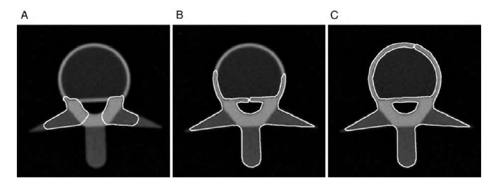
Figure 6.12 demonstrates the evolution of a topology-adaptive snake. The object is a CT cross section of a spine phantom, of which the edge image is shown in Figure 6.11. Initially, two snakes that have been placed near the vertebral processes start to expand, seeking the edges (part A). The two snakes intersect below the spinal canal and merge. The resulting single snake self-intersects and splits off a small snake that encloses the spinal canal (part B). The major snake expands along the vertebral cortex until it self-intersects near the apex of the vertebra and splits off a third snake that encloses the vertebral spongiosa (part C).

FIGURE 6.11 Edge image of a CT slice of a spine phantom with a grid of triangular cells superimposed.

FIGURE 6.12 Evolution of topology-adaptive snakes along the edges of a CT image of a spine phantom. (A) Two snakes start expanding and seeking the phantom edges. The snakes will intersect below the spinal channel and merge. (B) Above the spinal channel, the snake self-intersects and splits off a snake enclosing the spinal canal. (C) The dominant snake self-intersects again near the apex of the vertebra and splits off a third snake that encloses the spongy bone area, resulting in a total of three snakes.