The live wire is a highly interactive segmentation technique, aimed at aiding the user delineate an object boundary. The user selects a start point on the boundary. As the user hovers over the image with the mouse, the live wire tries to connect both points with an energy-minimizing path. The live wire tends to snap onto image edges. If the user is satisfied with the live-wire selection, the endpoint under consideration can be fixed and becomes the start point for the next segment. A live wire can be used to parametrize a path (e.g., a sulcus in a brain tomography image) or a closed contour. In the latter case it is possible to convert the live wire into a snake and continue with a snake algorithm for further processing.
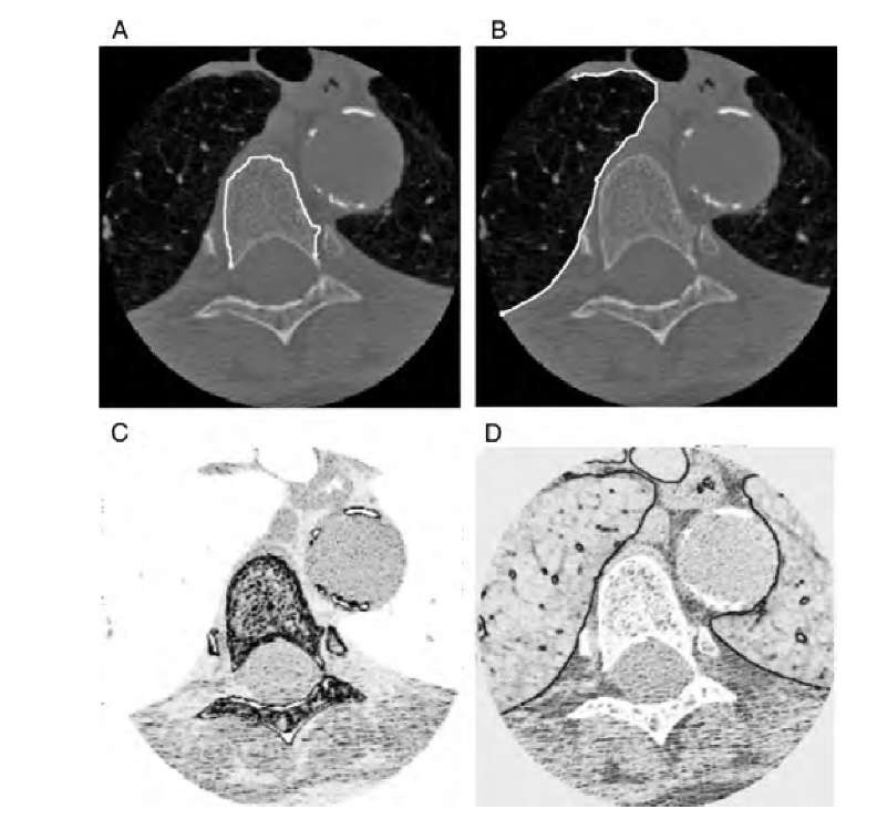
In the context of live wires, the energy function is referred to as the cost function. The principle of minimizing an energy or cost functional are the same. Apart from the higher level of user interaction, there are two more differences between live wires and snakes. First, the live wire is a path between start and end vertices with a global cost minimum. This is a consequence of the second difference, that is, the formulation of a live wire as a graph. Cost functions have even more parameters and user-definable features than the energy functions of a snake, therefore, a training step generally precedes the actual segmentation. The training step automatically adjusts numerous parameters to minimize the cost function for the specific type of edge to be segmented. An example is given in Figure 6.14, where a live wire was used to segment features in a chest CT image. First, the live wire was trained to detect the relatively low-contrast edge of the vertebral cortex (part A). The associated cost function (part C) shows low-cost values (dark shades) predominantly in the vertebral region and in regions of similar contrast. When trained for the high-contrast edge of the lung (B), the cost function looks different (D). In this case, edges of very high contrast show the lowest cost (darkest shades). When the live wire is trained for the lung edge, the vertebral edge actually repels the live wire. The ability to get trained for a specific type of edge contrast and width combined with the flexibility to set an arbitrary number of waypoints (intermediate end vertices that become the start vertex of a new segment) make the live wire a very flexible interactive tool for boundary delineating and segmentation.
FIGURE 6.14 Examples of live wires (white curves beginning with a circle and ending in an arrow) following the cortex of a vertebra (A) and the lung boundary (C) in chest CT images. Images B and D show the corresponding cost functions after training, where dark shades indicate low-cost pixel boundaries, and light shades indicate high-cost boundaries. Interpreted as valleys, the low-cost boundaries attract the live wire, which tries to follow the lowest-cost path.
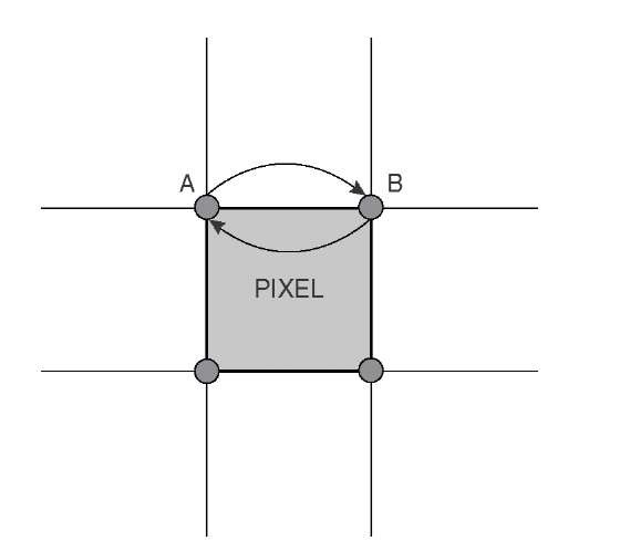
The live-wire model was introduced by Falcao et al.12 The key to this model is the interpretation of each boundary between two pixels of an image as a graph arc and each corner of a pixel as a graph node. This configuration is sketched in Figure 6.15, which shows one pixel and its four nodes, which are shared with the neighboring pixels. Two nodes are labeled A and B, and a boundary exists that connects A and B. The boundary is actually a vector, and the boundaries A ^ B and B ^ A are not identical. Every boundary (i.e., each arc of the graph) gets assigned a set of features that will later be used to compute the cost. The process takes place in two steps. First, a cost image (Figure 6.14C and D) is computed that stores the cost for each boundary. This cost image may later be modified by the training process. Second, from the user-selected start pixel P(x,y), the optimum path is computed for each pixel in the image, resulting in two two-dimensional arrays, the cumulative cost for the optimum path from the start pixel to each pixel in the image, and a two-dimensional array of directions indicating the immediate neighbor along the optimum path. The algorithm to obtain the arrays that contain the optimum path is explained below.
FIGURE 6.15 Interpretation of the image as a graph. Each pixel corner is a node (circle), and each pixel boundary that connects two nodes is a directed arc.
With the mouse hovering over any arbitrary pixel, the shortest path to the start pixel P(x,y) can be found extremely fast by following the negative directions in the two-dimensional array of directions. This path can be displayed in real time, thus providing the main interactive element: The user can observe—in real time—where the active contour lies with respect to the image features and can add control points if necessary.
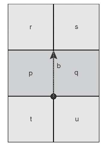
To understand the live wire algorithm and many related algorithms, two issues need to be considered: how to relate image features to cost, and how efficiently to find the lowest-cost path between two pixels of the image. To relate image features to cost, Falcao et al. proposed simultaneous use of eight feature functions12 that are related to either image intensity or image gradients. Assume a directed boundary b between pixels p and q, where p lies on the left side of b and q on the right side. Feature functions f 1 and f 2 are simply the image intensity values of pixels p and q, respectively. Feature function f 3 is the magnitude of the difference between f 1 andf2 (i.e., the absolute value of the gradient across the boundary b). Assuming the neighborhood definitions of the boundary b in Figure 6.16, feature functions f4, f 5, and f6 emerge as slightly different formulations of local gradients:
FIGURE 6.16 Definition of the pixel neighborhood of a boundary b.
Whereasf3 through f 6 are scalar values,f 7 is an oriented magnitude, defined as +f 6 if the direction of the gradient remains consistent with respect to the boundary direction and —f 6 otherwise. An alternative and maybe more intuitive formulation would be the definition of f5 without the magnitude function, that is,
The idea behind feature function f7 is to force the live wire to stay on the same side of a slope. For example, if the gradient is positive (when walking along the boundary in the direction of the arrow, image values go uphill from left to right), the cost associated with f7 is low. If the direction of the gradient changes, and the hill (positive gradient) is on the left side, the cost will go up.
Finally, feature function f 8 is the projected distance from a previously accepted live wire in a different image slice or in a previous image frame. Function f8 exists only if (1) the user analyzes a stack of images (either a three-dimensional image or a sequence of images evolving over time), (2) the evolution of the feature between successive slices is small, and (3) one initial slice has already been segmented.
The values of the feature functions are now converted to costs by means of cost functions, also called feature transforms. Six feature transforms, c1(f) through c6(f) have been proposed,12 and the final cost of a boundary b, c(b), is the weighted sum of all six cost functions, in its most general form,
Equation (6.45) reflects the notion that any feature function can be used with any feature transform. The weight factors wij make it possible to emphasize one feature function over others.
The individual feature transforms are defined by the following mapping functions. Mapping function c1 linearly maps the interval [l1,h1] of the feature value to the interval [0,1]. Values of f above h1 are clamped to 1, and values below l1 are clamped to 0. The inverse linear mapping function c2 can be defined as c2 = 1 – c1. It is possible, however, to use a different interval [l2,h2]. Mapping function c3 is a Gaussian function with the constant mean value f0 and the standard deviation ct. Mapping function c4 is an inverted Gaussian function, for example c4 = 1 – c3, where mean and standard deviation may differ from c3. Finally, mapping functions c5 and c6 are clamped hyperbolic functions with c6 = 1 – c5 and c5 defined as
Again, c5 and c6 do not necessarily use the same threshold values l3 and h3. Here a is a variable parameter that represents the focus of the hyperbola from its asymptotes, l3 is the distance of the vertical asymptote from the origin, and h3 is the upper cutoff value. Each pair of mapping functions provides a different emphasis. The Gaussian functions c3 and c4 provide high and low costs, respectively, for values near the center of the interval. The hyperbolic functions c5 and c6 provide a strong cost emphasis for the extrema of the interval.
The flexibility introduced with eight feature functions and six mapping functions is impractical, with each mapping function providing at least two variable parameters. Imagine a user interface where each parameter is represented by a user-modifiable slider. In the extreme case, this user interface would present the user with 14 parameters for the individual feature transforms and 48 weight parameters. In practical implementations, only a few combinations of feature functions, mapping functions, and their respective parameters will be used. Furthermore, some parameters can be assigned or refined through the training process, which is described below.
The next step in the live wire implementation is the algorithm to determine the lowest-cost path from the start pixel P(x,y) to each pixel of the image. The problem of finding the shortest path in a graph has been given much attention in the literature, and in conjunction with live wire implementations, Dijkstra’s algorithm11 is most frequently used. Most fundamental to the optimum path search algorithm is the property of optimum subpaths. If an optimum path from node P to node Q goes over node S, the path from P to S must also be the optimum path. Taken to the pixel level, the path from the starting point P(x,y) to any arbitrary endpoint Q(x,y) in the image plane consists of hops along the lowest-cost arc out of four possible choices from one pixel vertex to the next.
Dijkstra’s algorithm can be implemented with the following steps after it is provided with a starting vertex P.
Step 1. Create a data structure that contains, for each vertex v of the image, a cumulative cost cc(v), a direction for the optimum path to the immediate predecessor vertex, and a flag that indicates the processing status of vertex v. The direction may assume the values (U, W, N, E, S), where U stands for undefined. The flag may assume three values, (U, V, Q), where U stands for unprocessed, V stands for visited, and Q stands for queued. Step 2. Initialization: All cumulative cost values in the data structure are set to infinity (a very high value) except the cumulative cost associated with the starting vertex, which is set to zero. All status flags are set to U (unprocessed). All directions associated with the vertices are set to U (undefined). Step 3. Begin iteration: For vertex P, set its status flag to Q (queued). Step 4. Iteration: As long as there are queued vertices, repeat steps 5 through 8. Step 5. From all vertices that are queued, pick the one with the lowest associated cumulative cost. This is now vertex v;. Change the status flag of v; from Q to V. Step 6. Examine all four neighbors of v;: Perform steps 7 and 8 for each of the four neighbors provided that its associated flag has the value U. The neighbor under consideration is vj.
Step 7. Compute a temporary cost cT = cc(v,) + cost(vj ^ v;), which is the cumulative cost of vertex v; plus the cost of reaching v; from vj. Step 8. If cT < cc(vj), (a) update the cost cc(vj) = cT and set the direction of vj to point to v;, and (b) set the status flag of vj to Q. Step 9. The iteration ends when no vertices are flagged with a Q (i.e., the queue is empty).
At the end of Dijkstra’s algorithm, a cost structure exists for each pixel in the image. The cost functions described earlier come into play in step 7, where the cost of one arc (represented by the function cost vj ^ v;) is added to the cumulative cost of an existing path. There are modifications of the algorithm above which make use of ordered lists to reduce the time needed to search for the queued vertex with the lowest cumulative cost. The algorithm described above is a good starting point and is sufficiently efficient for most applications, considering that the algorithm is only executed every time a new starting point is selected. Once the algorithm has finished, the lowest-cost path from any arbitrary point in the plane to the start point P is found simply by following the directions stored with each vertex. This is an extremely fast process which allows updating the path in real time.
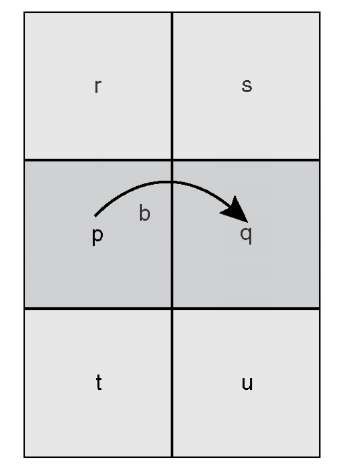
Another variation of the algorithm uses the pixel centers rather than the corners as nodes. In essence, this moves the grid by 1 pixel in each direction and uses an arc that goes from pixel center to pixel center. Here the feature functions need to be adjusted to reflect the fact that an arc no longer coincides with a pixel boundary. Using the definitions in Figure 6.17, feature functions f1 and f2 could be represented by the averaged intensities in pixels r and s, and t and u, respectively. Feature functions f3, f4, and f 5 are now identical and are the magnitude of the difference between f 1 andf2. Feature function f6 now becomes the average of the absolute difference between the intensities of r and u, and t and s, respectively, but it is doubtful whether this feature function would cause a measurably different behavior of the live wire from f 3. Finally, feature function f 6 is the simple difference between f 1 and f 2, so that the gradient direction can be considered. With the function f8 unchanged, the number of feature functions is now reduced to five. This variation reduces the level of complexity at the expense of some of the ability to follow extremely thin structures.
FIGURE 6.17 Definition of a pixel neighborhood for a center-to-center arc.
The last aspect of the live wire technique to be considered is the training process. Ideally, training is based on a set of user-selected points that represent typical feature properties. Once a segment of the live wire is established and the user is satisfied with the behavior of the live wire, the system may be retrained to include a larger number of points, and ideally, also directions. Unfortunately, for the large number of freely selectable parameters, no straightforward training scheme exists. For a single image feature and a single cost function, a least-squares approach to determine suitable parameters from several user-selected points may be used, but the complexity of this approach increases unacceptably with additional feature and cost functions. Arguably the most important mapping functions are the Gaussian mapping functions, because they can be trained to minimize the cost for any gradient strength. An example was given in Figure 6.14, where the bone-tissue interface shows a lower gradient than the lung-tissue interface. In regard to the Gaussian mapping function, the cost minimum (the mean of the inverted Gaussian function c4) would match the gradient strength. If the boundary is very homogeneous, a small standard deviation may be chosen. In fact, the live wire shows very good detection of features with intermediate contrast when only the Gaussian mapping function is used and the following training steps are taken.
Step 1. The user selects four to eight points along one representative boundary. For each point, the values of feature function f3 are collected, and their mean and standard deviation is computed. These values are used as initial trained values f0 and a for mapping function c4. Step 2. Based on the values of step 1, a live wire is drawn. Once the user accepts the course of the live wire, mean and standard deviation for feature function f3 for all pixels along the present live wire are computed and used as new values for f 0 and a. Step 3. Optionally, the user may, in a separate training step, select a number of points that do not represent the boundary. For these points the minimum and maximum values are computed and used as threshold values in the hyperbolic cost functions c5 and c6. By adding contributions from these cost functions, points that are an unlikely part of the contour sought make the path more expensive and therefore repel the live wire.
An alternative feature mapping technique was proposed by Marx and Brown.20 Here, two equally weighted inverse Gaussian mapping functions (c4) are used in conjunction with feature functions f 1 andf2. During the training step, values for f 1 and f2 are sampled, and the mean and standard deviation values are used as values f0 and a in the Gaussian mapping functions. Clearly, the effort to experiment with several different combinations of feature functions and mapping functions pays off when an optimum combination for a specific application is found.
The specific feature function f8 was mentioned briefly. This function may be used when advancing frame by frame in an image sequence or when using the live wire to move through a three-dimensional image stack. Feature function f8 makes the path more expensive when it deviates more strongly from the path chosen in the previous frame or slice. A more advanced technique was proposed by Marx and Brown.20 For progression through image slices or successive image frames, the closed-contour live wire is converted into a snake. For this purpose, snake vertices are sampled along the live wire with a curvature-dependent density. The snake is allowed to converge on the next slice and gets converted back into a live wire by performing a training run along the snake contour. A related technique for the progression from slice to slice was presented by Salah et al.24 In this variant, the live wire control points (the start points of the segments) are reexamined upon progression to the next slice. To advance to the next slice, the local neighborhood of the control points is examined for the cost minimum according to the cost function selected, and the control points are then moved to the new minimum. This method that can be implemented with an unsupervised algorithm. After moving the control points, the live wire searches the optimum path between the control points by using conventional methods. The live wire concept can also be extended into three-dimensional by a different technique, proposed by Hamarneh et al.14 The basic idea is to use seed points in different slices to create orthogonal live wires. Points along the mesh of live wires generated by this method can be sorted to generate meaningful additional (and automatically generated live wires) that eventually provide the contour of the three-dimensional object being segmented.
Live wires are designed to find the globally optimal path. However, it is possible to combine the path cost term with an internal cost term, analogous to the internal energy of a snake.15 The inclusion of an internal energy term requires extension of Dijkstra’s optimum path search algorithm to three dimensions. With the well-known weight parameters a and p for stretching and curvature, the modified live wire, termed a G-wire, tends to follow a smoother path and can be prevented from digressing to neighboring similar features.


