The Fourier transform and its properties were discussed in topic 3. Of particular importance is the property of edges, boundaries, and irregularities in general to correspond to broadband frequency components. The underlying principle that allows a definition of a fractal dimension in the frequency domain is the question: How fast does the amplitude of the signal or image drop off toward higher frequencies? Intuitively, the frequency transform of an image with smooth features would show a steeper drop-off toward higher frequencies than would an image with many discontinuities and irregular features. Once again, the analysis of random processes lends itself to a rigid definition of the fractal dimension in the frequency domain. If the source of a random process produces values that are completely independent of each other, the random sequence is referred to as wh te no se. White noise has uniform local properties (i.e., its mean and standard deviation within a local window are widely independent of the window location). More important, white noise has a broadband frequency spectrum. In other words, each frequency has the same probability of occuring over the frequency range observed. In many random processes, however, consecutive samples are not completely independent. Rather, a trend can be observed that an increased value from one sample to the next is followed by a higher probability of additional value increases, an effect called pers stence. The source is said to have a memory.
The origins of the analysis of the fractal dimension in the frequency domain lie in the analysis of random time series. H. E. Hurst observed water levels of the river Nile and found long-term dependencies (i.e., persistence). Moreover, Hurst found that the range of the water level scales with the duration of observation.28 If the range R is defined as the difference between the highest level Lmax(T) and the lowest level Lmin(r) in an observational period of length t and ct is the standard deviation of the river levels during the period t , then the range shows a power-law dependency on the length of the observational period:
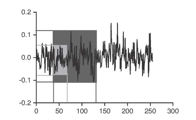
This scaling behavior of discrete time samples was found in many other areas, such as in financial data52 and biology. One biomedical example is the potassium channel in pancreatic (-cells, where the opening and closing of the channels has been found to exhibit self-similar properties.41 Moreover, the opening and closing of the channels have been found to exhibit memory effects, where an opening of the channel is followed by a higher probability of the channel opening again.38 A scaling behavior as described in Equation (10.14) generally pertains to random events with a certain long-term memory. Such a series of events has been approximated with the model of fractional Brownian noise. For completely uncorrelated noise (white noise), H = 0.5, whereas persistence in the random time series yields H > 0.5 and antipersistence yields H < 0.5. A time series with persistence appears smoother. Equation (10.14) can be used to estimate the Hurst exponent from sampled data. Figure 10.20 demonstrates this process.
With a growing observational window, the window is more likely to contain extreme values, and the range R can be expected to grow. In the time domain, the scaling factor is estimated by rescaled range analysis. The time series of total length T is subdivided into n = T/t observational windows of length t . For each window, the rescaled range (minimum to maximum normalized by the standard deviation in that window) is determined and averaged. Iteratively, a new, longer t is chosen and the average rescaled range is determined again. From a number of ranges Ri (T ) obtained at different window lengths T , the scaling exponent H is obtained by nonlinear regression. The Hurst exponent is related to the fractal dimension by D = 2—H. This relationship is based on the scaling behavior of the amplitude of the Brownian time series and may not be valid for all time series. However, this relationship has been widely used and may be considered to be established.
FIGURE 10.20 Random time series and two observational windows. A larger window (dark shade) has a higher probability of containing local extremes; therefore, the range (difference between highest and lowest value) is likely to be higher than in the shorter window (light shade).
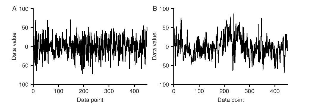
FIGURE 10.21 Uncorrelated Gaussian noise (A) and persistent noise of zero mean and matching standard deviation (B). Persistent noise exhibits large-scale, low-frequency trends and additional trends on smaller time scales and smaller amplitudes.
Figure 10.21 shows two random time series of matching mean and standard deviation. Persistent noise (Figure 10.21B) exhibits trends on all time scales, and self-similar behavior can be expected. Conversely, uncorrelated Gaussian noise (Figure 10.21A) does not obey a scaling law. We have already quantified persistence by means of the Hurst exponent, which characterizes scaling behavior in the time domain. Low-frequency trends and scaling behavior can also be seen in the frequency domain: As opposed to broadband white noise, low frequencies dominate for persistent noise. More precisely, a time series that exhibits scaling behavior as described in Equation (10.14) also follows the frequency-domain scaling behavior described by,
where A is the amplitude of the frequency spectrum and w the frequency. The negative sign in the exponent indicates an amplitude decay with higher frequencies. The scaling exponent, p, is related to the Hurst H exponent through
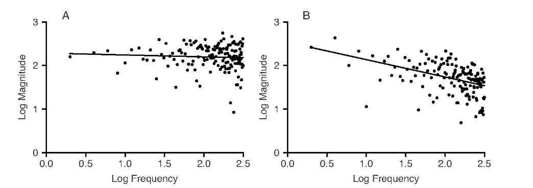
where DE is the Euclidean dimension on which the signal is built (i.e., 1 for a time series and 2 for a two-dimensional image). The scaling exponent p in Equation (10.15) can be determined by fitting a regression line into the log-transformed data points of the spectral magnitude over the frequency as shown in Figure 10.22.
FIGURE 10.22 Magnitude of the frequency spectra of the signals in Figure 10.21. Uncorrected Gaussian noise (A) shows no significant decay of the magnitude at higher frequencies (regression line: slope not significantly different from zero), whereas persistent noise (B) shows power-law scaling with decreasing amplitude at higher frequencies. The slope is ( = 0.52 (p < 0.0001) which is in excellent agreement with the Hurst exponent of H = 0.75 determined for the corresponding series in Figure 10.21.
There are some special cases of ( . Uncorrelated noise exhibits no frequency dependency of the spectral magnitude, and the slope (is not significantly different from zero. From Equation (10.16) follows H = 0.5, that is, the Hurst exponent associated with uncorrelated (white) noise. If the magnitude decays inversely proportional to the frequency (( = —1), the noise is referred to as 1f noise or pink noise. An even steeper decay, 1/f2 (( = —2), is obtained from data series that originate from Brownian motion or random walks and is termed brown or red noise.
Similar to the estimators of the fractal dimension, the regression to determine ( needs to be restricted to frequencies in which self-similar behavior can be expected. The presence of measurement noise can lead to apparent multifractal behavior where the magnitude at high frequencies decays with a different slope than the magnitude at low frequencies. A lowpass filter (such as Gaussian blurring) applied to white noise may lead to a spectrum that resembles pink noise, but it would not originate from a process with inherent scaling behavior.
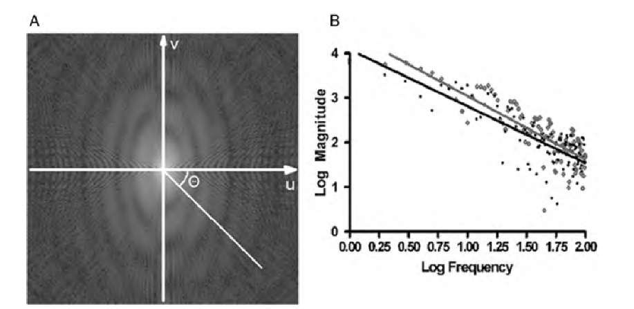
The considerations described above can easily be extended to images. However, images may exhibit different spectral behavior, depending on the angle at which the spectrum is examined. Circles around the origin of a Fourier transform image connect locations of equal frequency, because the frequency w increases with the Euclidean distance from the origin![]() As seen in Figure 10.23,spectra sampled along the u-axis and along a diagonal line starting at the origin look different and exhibit a different scaling exponent ( . Multifractal behavior of Fourier transform images is therefore very common. In an extreme example, features with straight edges parallel to the y-axis and rugged edges along the x-axis would exhibit scaling behavior along the u-axis but not along the f-axis. Because of this complex behavior, the most common use of fractal analysis of Fourier transform images is to identify anisotropic fractal behavior. For this purpose, the scaling exponent ( is computed along one-dimensional spectra subtending various angles 0 with the u-axis.
As seen in Figure 10.23,spectra sampled along the u-axis and along a diagonal line starting at the origin look different and exhibit a different scaling exponent ( . Multifractal behavior of Fourier transform images is therefore very common. In an extreme example, features with straight edges parallel to the y-axis and rugged edges along the x-axis would exhibit scaling behavior along the u-axis but not along the f-axis. Because of this complex behavior, the most common use of fractal analysis of Fourier transform images is to identify anisotropic fractal behavior. For this purpose, the scaling exponent ( is computed along one-dimensional spectra subtending various angles 0 with the u-axis.
FIGURE 10.23 Frequency spectra observed at different angles in the Fourier transform of an image. Along the u-axis (gray data in the log-log plot), the frequency drops off faster than along a diagonal line of angle 0 (black data in the log-log plot).
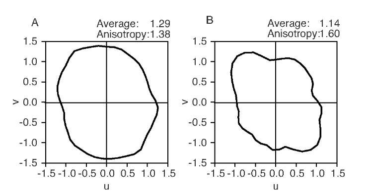
The resulting function p(0) can be displayed in the form of a rose plot. The information provided by a rose plot can be shown using two sample textures that were introduced in topic 8 (see the carpet and corduroy textures in Figures 8.10 and 10.28). Their fractal rose plots are shown in Figure 10.24. The average slope p is 1.29 for the carpet texture and 1.14 for the corduroy texture. However, the anisotropy, defined as the maximum value of p divided by the minimum value of p, is markedly higher for the corduroy texture, indicating a higher directional preference. In addition, the angle of the anisotropy (the orientation of the idealized oval) of approximately 120° matches the orientation of the texture. The rose plot is therefore a convenient method to use for the quantitative determination of the anisotropic behavior of textures with self-similar properties. In addition to the average slope (, anisotropy magnitude, and angle, the intercept of the fit may be used to measure anisotropic behavior of the image intensity itself.
FIGURE 10.24 The slope of the double-logarithmic frequency decay of two textures from topic 8 (carpet, A, and corduroy, B, also shown in Figure 10.28), displayed as a function of the angle in form of a rose plot. The slopes (and therefore the Hurst exponents) are somewhat similar, but the corduroy texture (right) shows a higher anisotropy than the carpet texture, because the original texture has a stronger directional preference. The anisotropy angle of 120° also matches the directional preference of the texture in Figure 10.28.
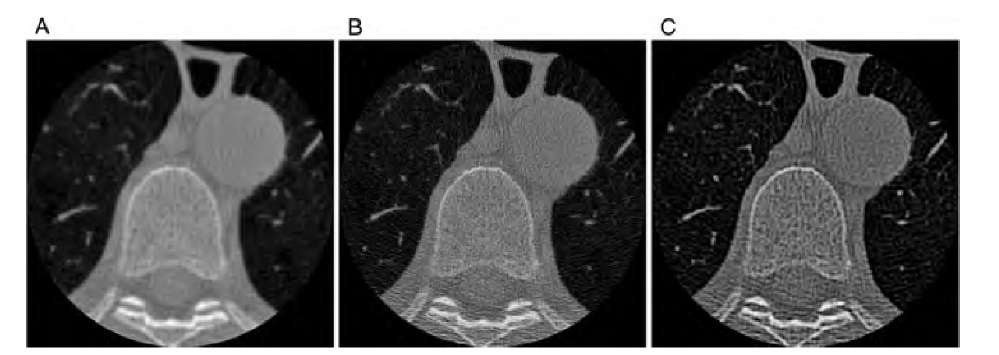
FIGURE 10.25 CT reconstructions of the thoracic region using different reconstruction kernels: (A) standard kernel, (B) bone kernel, (C) lung kernel. The reconstruction kernels emphasize different levels of detail, but they also create a pseudotexture with apparent fractal properties.
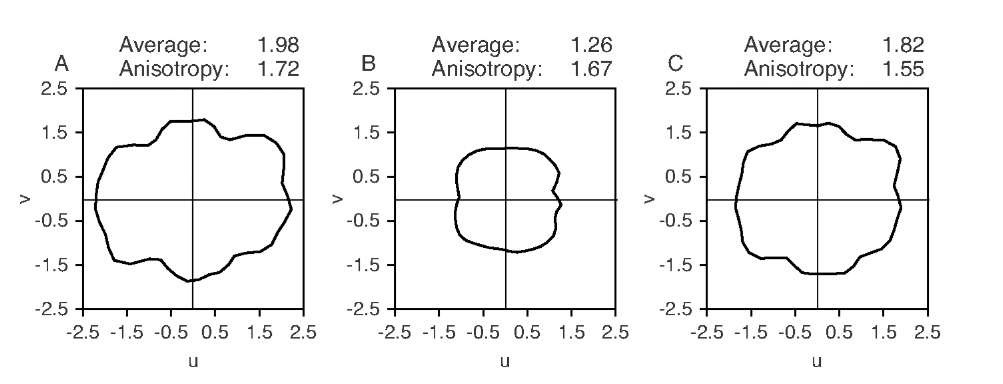
Figure 10.25 shows cross-sectional CT images of the thoracic region, that make possible easy identification of lungs, vertebra, and aorta. Corresponding rose plots are shown in Figure 10.26. The three panels show reconstructions performed with different reconstruction kernels: the standard kernel, the bone kernel, and the lung kernel. The purpose of these kernels (i.e., filters applied during reconstruction) is to emphasize specific details in the region of interest.
FIGURE 10.26 Rose plots of the frequency decay behavior of the CT reconstructions in Figure 10.25. The rose plots indicate strongly differing apparent self-similar behavior among the three CT images.
Although the reconstruction was performed using the same raw data, apparent fractal properties are markedly different. The texture that causes the apparent self-similar properties is a CT artifact. This can best be observed in the region of the aorta, where homogeneous blood flow should correspond to a homogeneous gray area in the reconstruction. In actual reconstructions, however, the aorta cross section is inhomogeneous, and the inhomogeneity depends on the reconstruction kernel. A linear regression into log-transformed data, in this case the logarithmic spectral amplitude over the logarithmic frequency, will often lead to a reasonable approximation of a straight line, but a thorough discussion of the origins of possible self-similar properties is needed in all cases.

