Managing Uncertainty in a Geospatial Model of Biodiversity Part 2

Distance from ridgeline

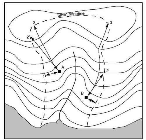
The distance from ridgeline (DFR) variable was used as a surrogate for moisture and nutrient gradients which are a result of hillslope process. Estimates of the distance from each image pixel to the nearest ridgeline were required. The algorithm (path 2 in Figure 11.4) for estimating this variable was a compromise between the shortest Euclidean distance (path 1 in Figure 11.4) (Bridge, 1997) and the continuous path that crosses each elevation contour at right angles (path 3 in Figure 11.4).

Table 11.2 Summary of kNN results for testing sites using (a) 7 band Landsat TM data and (b) SIR-C SAR data. In each matrix the rows indicate the label in the reference data while the columns that in the classified image. Note that due to incomplete overlap of the SAR and TM data sets the sample size differs slightly

Class	JP	BS	TA	MIX	WAT	ANT	WET	Kappa
JP	173	2	26	15	0	0	3	0.78
BS	14	43	0	75	0	0	0	0.31
TA	6	0	335	9	0	0	1	0.95
MIX	10	16	13	61	0	0	0	0.59
WAT	0	0	0	0	2018	0	0	1.00
ANT	1	0	32	0	0	397	50	0.80
WET	19	4	27	0	0	117	544	0.72
(a)

Class	JP	BS	TA	MIX	WAT	ANT	WET	Kappa
JP	67	25	74	4	0	49	0	0.25
BS	31	68	6	6	0	15	6	0.48
TA	55	25	204	17	0	11	4	0.60
MIX	18	37	6	30	0	9	0	0.28
WAT	0	0	0	0	788	0	0	1.00
ANT	35	41	39	11	0	336	17	0.63
WET	0	4	1	0	0	113	593	0.79
(b)

Table 11.3 Summary of classification results after SAR and TM classifications were combined. The rows indicate the label in the reference data while the columns that in the classified image. The change in kappa coefficient, relative to that derived to the use of the TM data alone is also shown

Class	JP	BS	TA	MIX	WAT	ANT	WET	kappa	Change in kappa
JP	164	6	36	9	0	1	3	0.73	-0.05
BS	17	61	2	40	0	6	6	0.44	+0.13
TA	1	0	312	1	0	0	2	0.99	+0.04
MIX	10	20	17	50	0	3	0	0.50	-0.09
WAT	0	0	0	0	788	0	0	1.00	0
ANT	1	0	39	0	0	408	32	0.85	+0.05
WET	0	1	12	0	0	141	557	0.78	+0.06

Figure 11.4 Three possible approaches for measuring distance from two pixels (A and B) to a basin ridgeline. The first (used by Bridge (1997)) finds the closest ridge. The second (from this work) finds the closest ridge based on a path direction calculated from local aspect. The third traces a path which cuts perpendicularly through contour lines and is considered to be the best estimate

Calculation of DFR was subject to many sources of uncertainty. For the DEM, these sources include uncertainty from the contour lines used for interpolation, the errors produced during interpolation and resampling the grid cell size. For the basin and ridge delineation, these sources include uncertainty from the flow direction and flow accumulation. Uncertainty was also introduced in calculating the distance from the ridgelines. In some situations, there were no river vectors to ensure that a basin was properly divided such that distances would only be measured from a pixel to its respective ridge.

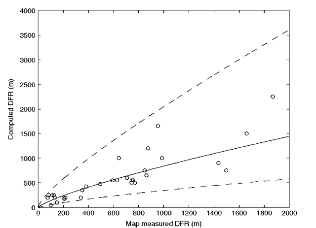
The quantity and qualitative nature of the uncertainties present in the data and processes used to calculate DFR made it impossible to model the uncertainty in the DFR. The assessment of uncertainty for the DFR map, therefore, was of an empirical nature. A comparison data set consisting of manually measured DFR from 1:50 000 topographic maps was acquired for each of the sampled forest stands. Uncertainty in the DFR data was assessed by comparing the values estimated manually from the maps with those computed algorithmically. For this, forest stands were located on the topographic maps and from a visual assessment of the terrain around a forest stand, the nearest ridge was located on the map and the distance measured. The measured transect running from stand up to ridge always cut perpendicularly through the contour lines. This was repeated for 31 forest stands such that a full range of distances were sampled. Figure 11.5 shows the relationship between map-measured DFR and computed DFR. The dashed lines are the 95 % confidence intervals which were used as estimates of DFR uncertainty.

Figure 11.5 The correlation between the two methods used to determine DFR for 31 ground sample forest stands. For the manually calculated method, 1:50 000 topographic maps were interpreted and basin ridgelines were traced out. The distance was measured from forest stand to ridge by cutting a path perpendicularly through contours. Included on the plot is the loglinear regression line and error bars (dotted lines) based on a 95 % confidence level

Canopy stem density

Estimating canopy stem density (CSD) from satellite sensor imagery was extremely difficult. Reports of canopy stem density estimates for boreal forest are sparse in the literature. Many studies have demonstrated the use of SAR to predict forest characteristics such as species composition, biomass, leaf area index (LAI) or diameter at breast height (DBH) (Ranson et al., 1995; Ranson and Sun, 1994; Le Toan et al., 1992; Wilson, 1996). However, within this literature there is little or no attention given to the estimation of stem density. It seems plausible that estimation of stem density has been largely unsuccessful and thus, reporting of results has not followed.

Kurvonen et al. (1999) estimated stem volume using L-band JERS-1 and ERS-1 SAR data. However, their prediction equations required the use of vegetation and ground moisture and were not practical for this work.

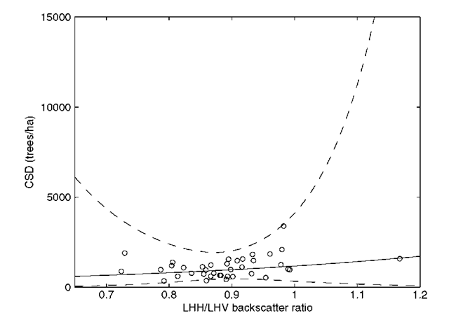
Ranson et al. (1995) and Ranson and Sun (1994) found correlations between SAR band ratios and forest biomass. They proposed that using a ratio of SAR bands (as opposed to unratioed bands) may increase signal dynamic range and thus increase the correlation with forest properties. Ranson et al. (1995) related the logarithm of forest biomass to SIR-C SAR LHV backscatter with a coefficient of determination (R2) of 0.846 for the BOREAS study site which is adjacent to PANP, but such results were not reproduced at this site. Collins and Livingstone (1996) used SAR polarization ratios (same band) for mapping thin sea ice. These techniques were examined for this research: all possible combinations of SAR polarization and band ratios were regressed with the natural logarithm of canopy stem density. The L-band polarization ratio (LHH/LHV), had the largest, although still small, correlation coefficient with CSD (R2 = 0.13). The basic form of the model relationship was:

and the relationship is depicted graphically in Figure 11.6. To determine the error interval, the ln(error) was added and subtracted from the ln(CSD) to gain the upper and lower error bounds on the prediction. The exponential of each was then calculated which produced the error in terms of CSD. These bounds are plotted in Figure 11.6 as the dashed lines. An important feature to notice is that the error bounds are not symmetric about the prediction value. This is a product of using logarithmically transformed data in the model development. As can be seen in the graph SAR input values below 0.8 and above 1.0 are prone to extremely high uncertainty.

Uncertainty propagation

The parameters in the linear model were estimated using field observations of richness, DFR, TSF, canopy species type and CSD. The model parameters are listed in Table 11.4, note that the model is in reality four models with the delta values (S) changing the slope for each canopy type.

An outline of the overall richness estimation procedure is given in Figure 11.2. To produce a map of estimated richness, the model was run for each pixel using the estimates of the DFR, CSD and TSF. The canopy type classification algorithm generated a vector of class membership likelihoods for each pixel. We summed the likelihoods for the four forest classes and if this sum was greater than a threshold the pixel was determined to be a forest pixel otherwise it was labelled with one of the three non-forest classes.

Table 11.4 Parameter estimates for the species richness equation (equation (1))

Term	Estimate
	25.995261
	-0.036611
	-0.000926
	-0.004021
	0.8042173
	-4.295932
	4.7861226

For a pixel labelled as forest, the richness model was run four times, once for each of the canopy types, and derived a weighted average richness in which the weights were the class likelihoods for the forest classes as follows,

where pi are the class likelihoods.

The uncertainties for DFR and CSD are non-symmetric confidence intervals derived from regressions of estimates against observations. The uncertainties for TSF are symmetric intervals in the interior of the TSF polygons and non-symmetric upper and lower bounds in the polygon boundary zones. There was no straightforward way to propagate these disparate errors through the model. We decided, therefore, to be conservative and use upper and lower bounds on the richness as our estimates of uncertainty for our richness predictions. These two bounds represent two worst-case scenarios when we have all the errors adding together rather than cancelling each other as normal error analysis assumes. Note that given the negative values for fl 1…3, S increases in value with a decrease in CSD, DFR and TSF. Hence, the lower bound on S was generated by using upper bounds on the three landscape variables in equation (1). As before, a weighted average lower bound was calculated. The same procedure was followed for calculating the weighted average upper bound on richness.

Figure 11.6 Measurement data and the linear regression model used to predict canopy stem density from the SAR backscatter ratio. The solid line is the model prediction line (of best fit) and the dashed lines represent error bars two standard deviations from the prediction line

Results and Discussion

The first result was intended to answer question 1: How well can richness be estimated using estimated versus observed landscape variables?

Figure 11.7 is a comparison between the richness predicted from the estimated landscape variables versus the richness predicted from the observed variables. The degree of correlation, while not particularly largeindicated that we should have some confidence in the predictive model when we apply it to the whole landscape.

Figure 11.7 Comparison of richness estimates: (a) the relationship between richness predicted using observed variables versus richness predicted from estimated variables, (b) the residuals, these are estimated – observed

Figure 11.8 Comparison of richness estimates: (a) the relationship between richness observed in the field with that predicted from the model, (b) the residuals from the relationship

The residual plot in Figure 11.7b shows that the estimated-variable prediction tends to over-estimate the richness relative to the observed-variable prediction (which is itself higher than the observed richness); the residual RMS error was 3.8 species. Hence, the effect of using estimated versus observed landscape variables in the richness model was to over-estimate richness.

The second question addressed was: How accurate are richness predictions relative to field observations? Figure 11.8 is a comparison between the richness predicted from the model versus the richness observed in the field. Again, the degree of correlation was relatively smallbut it was significant.

The residual plot in Figure 11.8 shows largely positive residuals (RMS error is 6.8 species) that indicated that the model tended to under-estimate the richness relative to the observed richness for the testing samples. Hence, the model was conservative in its estimation of richness.

Finally, the level of uncertainty in the richness predictions was evaluated. The error bars in Figure 11.8 are the upper and lower bounds on the estimated richness. There are two features to note. First, the size of the bars plotted. A consistently conservative approach to the estimation and propagation of error has been used and this led to very large levels of uncertainty in the richness estimates. This should not erode the value of the richness map. While the levels of uncertainty in the map are high they are at least quantified which is regarded as a step forward in biodiversity mapping. The second feature to note is that the errors are non-symmetric with the upper bound being larger than the lower bound. This is consistent with the finding that the estimated richness values were smaller than the observed values. The predicted richness was conservative which may be viewed as a positive result.

Figure 11.9 (see plate 6) shows a sample of the predicted species richness map for the PANP together with the upper and lower bounds. The wetter areas of the park tend to have lower diversity. This observation coincides with the reasoning for the inclusion of the distance from a ridgeline variable into the model. However, the actual patterns in the distance from a ridgeline occur at a finer scale than on the species richness map and, therefore, there are no apparent spatial correlations between the two maps. The same is true for canopy stem density. In general, areas which were classified as trembling aspen are highly correlated with relatively high biodiversity. Lower biodiversity areas tend to coincide with the spatial distribution of jack pine and the mixed class. The lowest biodiversity coincides with black spruce. There was no apparent spatial correlation between the patterns of species richness and the time-since-fire map. Since fire is suppressed within the park, there tends to be very little young forest area. This might account for the lack of apparent variation in species richness due to this variable.

Conclusions

This work has shown that a simple richness model is, to some extent, capable of estimating the correct levels of biodiversity in a variety of landscapes. The form of the uncertainties in the input landscape variables differ from one another making it impossible to implement standard methods of error propagation. In the absence of a standard solution a deliberately conservative approach has been used. A method for representing and propagating uncertainty through a predictive model for species richness was also developed and used. This has led to clear, if conservative levels of uncertainty. Nevertheless, by propagating and reporting uncertainty associated with a biodiversity map, a realistic understanding of the limits of both the resulting map and model itself have been obtained. This can prevent misuse of such a map and allows the refinement of the model inputs to reduce uncertainty.