Serial correlation is a statistical term that refers to the linear dynamics of a random variable. Economic variables tend to evolve parsimoniously over time and that creates temporal dependence. For instance, as the economy grows, the level of gross national product (GNP) today depends on the level of GNP yesterday; or the present inflation rate is a function of the level of inflation in previous periods since it may take some time for the economy to adjust to a new monetary policy.
sors such as unemployment and other macroeconomic variables. Under the classical set of assumptions, the Gauss-Markov theorem holds, and the ordinary least squares (OLS) estimator of the f3j’s is the best, linear, and unbiased estimator (BLUE). Serial correlation is a violation of one of the classical assumptions. Technically, we say that there is serial correlation when the error term is linearly dependent across time, that is, the cov(£ , £ ) ^ 0 for t ^ s. We also say that the error term is autocorrelated. The covariance is positive when on average positive (negative) errors tend to be followed by positive (negative) errors; and the covariance is negative when positive (negative) errors are followed by negative (positive) errors. In either case, a covariance that is different from zero will happen when the dependent variable Yt is correlated over time and the regression model does not include enough lagged dependent variables to account for the serial correlation in Yt . The presence of serial correlation invalidates the Gauss-Markov theorem. The OLS estimator can still be unbiased and consistent (large sample property), but it is no longer the best estimator, the minimum variance estimator. More importantly, the OLS standard errors are not correct, and consequently the t-tests and F-tests are invalid.
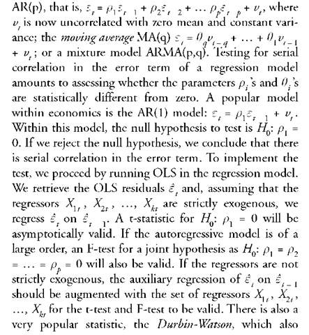
There are several models that can take into account the serial correlation of £t : the autoregressive model
requires strict exogeneity that tests for AR(1) serial correlation. The main shortcoming of this test is the difficulty in obtaining its null distribution. Though there are tabulated critical values, the test leads to inconclusive results in many instances.
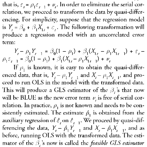
Once we conclude that there is serial correlation in the error term, we have two ways to proceed depending upon the exogeneity of the regressors. If the regressors are strictly exogenous, we proceed to model the serial correlation and to transform the data accordingly. A regression model based on the transformed data is estimated with generalized least squares (GLS). If the regressors are not exogenous, we proceed to make the OLS standard errors robust against serial correlation. In the first case, let us assume that there is serial correlation of the AR(1) type,
(FGLS), which is a biased estimator, though asymptotically is still consistent. In practice, the FGLS estimator is obtained by iterative procedures known as the Cochrane-Orcutt procedure, which does not consider the first observation, or the Prais-Winsten procedure, which includes the first observation. When the sample size is large, the difference between the two procedures is negligible.
In the second case, when the regressors are not strictly exogenous, we should not apply FGLS estimation because the estimator will not be even consistent. In this instance, we modify the OLS standard errors to make them robust against any form of serial correlation. There is no need to transform the data as we just run OLS with the original data. The formulas for the robust standard errors, which are known as the HAC (heteroscedasticity and autocorrelation consistent) standard errors, are provided by Whitney Newey and Kenneth West (1987). Nowadays, most of the econometric software calculates the HAC standard errors, though the researcher must input the value of a parameter that controls how much serial correlation should be accounted for. Theoretically, the value of this parameter should grow with the sample size. Newey and West advised researchers to choose the integer part of 4(T /100)2/9 where T is the sample size. Although by computing the HAC standard errors we avoid the explicit modeling of serial correlation in the error term, it should be said that they could be inefficient, in particular when the serial correlation is strong and the sample size is small.


