The term regression was initially conceptualized by Francis Galton (1822-1911) within the framework of inheritance characteristics of fathers and sons. In his famous 1886 paper, Galton examined the average regression relationship between the height of fathers and the height of their sons. A more formal treatment of multiple regression modeling and correlation was introduced in 1903 by Galton’s friend Karl Pearson (1857-1936). Regression analysis is the statistical methodology of estimating a relationship between a single dependent variable (Y) and a set of predictor (explanatory/independent) variables (X2, X3, … Xp based on a theoretical or empirical concept. In some natural science or engineering applications, this relationship is exactly described, but in most social science applications, these relationships are not exact. These nonexact models are probabilistic in nature and capture only approximate features of the relationship. For example, an energy analyst may want to model how the demand for heating oil varies with the price of oil and the average daily temperature. The problem is that energy demand may be determined by other factors, and the nature of the relationship between energy demand and explanatory variables is unknown. Thus, only an approximate relation can be modeled.
The simplest relationship between Y and X is a linear regression model, which is typically written as,
where the index i represents the i-th observation and U. is the random error term. The [ coefficients measure the net effect of each explanatory variable on the dependent variable, and the random disturbance term captures the net effect of all the factors that affect Yi except the influence of the predictor variables. In other words, U. is the difference between the actual and mean value
observations. The explanatory variables are assumed to be nonstochastic and uncorrelated with the error term. The meaning of the [ coefficient varies with the functional form of the regression model. For example, if the variables are in linear form, the net effect represents the rate of change, and if the variables are in log form, the net effect represents elasticity, which can be interpreted as a percentage change in the dependent variable with respect to a 1 percent change in the independent variable.
squares (OLS) method. The minimization problem results in k equations in k unknowns, which gives a unique estimate as long as the explanatory variables are not collinear. An unbiased estimate of a is obtained from the residual sum of squares. When the random error term satisfies the standard assumptions, the OLS method gives the best linear unbiased estimates (BLUE). The statistical significance of the coefficients is tested with the usual t-statistic (t = pi s.e.(pi)), which follows a t-distribution with n – k degrees of freedom. In fact, some researchers use this t-statistic as a criterion in a stepwise process to add or delete variables from the preliminary model.
The fit of the regression equation is evaluated by the statistic R2, which measures the extent of the variation in Y explained by the regression equation. The value of A2 ranges from 0 to 1, where 0 means no fit and 1 means a perfect fit.
compensates for n and k, is more suitable than R in comparing models with different subsets of explanatory variables. Sometimes researchers choose the model with the highest A2, but the purpose of the regression analysis is to obtain the best model based on a theoretical concept or an empirically observed phenomena. Therefore, in formulating models, researchers should consider the logical, theoretical, and prior knowledge between the dependent and explanatory variables. Nevertheless, it is not unusual to get high A2 with the signs of the coefficients inconsistent with prior knowledge or expectations. Note that As of two different models are comparable only if the dependent variables and the number of observations are the same, because A measures the fraction of the total variation in the dependent variable explained by the regression equation. In addition to R2, there are other measures, such as Mallows’s C statistic and information criteria AIC (Akaike) and BIC (Bayesean), to choose between different combinations of regressors. Francis Diebold (1998) showed that there is no obvious advantage between AIC or BIC, and they are routinely calculated in many statistical programs.
Regression models are often plagued with data problems, such as multicollinearity, heteroskedasticity, and autocorrelation, that violate standard OLS assumptions. Multicollinearity occurs when two or more (or a combination of) regressors are highly correlated. Multicollin-earity is suspected when inconsistencies in the estimates, such as high A2 and low t-values or high pairwise correlation among regressors, are observed. Remedial measures of multicollinearity include dropping a variable that causes multicollinearity, using a priori information to combine coefficients, pooling time series and cross-section data, adding new observations, transforming variables, and ridge and Stein-rule estimates. It is worthwhile to note that transforming variables and dropping variables may cause specification errors, and Stein-rule and ridge estimates produce biased and inefficient estimates.
The assumption of constant variance of the error term is somewhat unreasonable in empirical research. For example, expenditure on food is steady for low-income households, while it varies substantially for high-income households. Furthermore, heteroskedasticity is more common in cross-sectional data (e.g., sample surveys) than in time series data, because in time series data, changes in all variables are in more or less the same magnitude. Plotting OLS residuals against the predicted Y values provides a visual picture of the heteroskedasticity problem. Formal tests for heteroskedasticity are based on regressing the OLS residuals on various functional forms of the regressors. Halbert White’s (1980) general procedure is widely used among practitioners in detecting and correcting het-eroskedasticity. Often, regression models with variables observed over time conflict with the classical assumption of uncorrelated errors. For example, in modeling the impact of public expenditures on economic growth, the OLS model would not be appropriate because the level of public expenditures are correlated over time. OLS estimates of [3s in the presence of autocorrelated errors are unbiased, but there is a tendency for a to be underestimated, leading to overestimated A2 and invalid t- and /-tests. First-order autocorrelation is detected by the Durbin-Watson test and is corrected by estimating difference equations or by the Cochrane-Orcutt iterative procedure.
SPECIFICATION ERRORS
The OLS method gives the best linear unbiased estimates contingent upon the standard assumptions of the model and the sample data. Any errors in the model and the data may produce misleading results. For example, the true model may have variables in log form, but the estimated model is linear. Even though in social sciences, the true nature of the model is almost always unknown, the researchers’ understanding of the variables and the topic may help to formulate a reasonable functional form for the model. In a situation where the functional form is unknown, possible choices include transforming variables into log form, polynomial regression, a translog model, and Box-Cox transformation. Parameters of the Box-Cox model are estimated by the maximum likelihood method because the variable transformation and the parameter estimation of the model are inseparable.
Specification errors also occur either when relevant explanatory variables are missing from the model or when irrelevant variables are added to the model. For example,
between the variables X2 and X3. In addition, incorrect estimation of a2 may lead to misleading significance tests. Researchers do not commit these specification errors willingly; often the errors are due to unavailability of data or lack of understanding of the topic. Researchers sometimes include all conceivable variables without paying much attention to the underlying theoretical framework, which leads to unbiased but inefficient estimates, which is less serious than omitting a relevant variable.
Instead of dropping an unobserved variable, it is common practice to use proxy variables. For example, most researchers use general aptitude test scores as proxies for individual abilities. When a proxy variable is substituted for a dependent variable, OLS gives unbiased estimates of the coefficients with a larger variance than in the model with no measurement error. However, when an independent variable is measured with an error, OLS gives biased and inconsistent estimates of the parameters. In general, there is no satisfactory way to handle measurement error problems. A real question that arises is whether to omit a variable altogether or instead use a proxy variable. B. T. McCallum (1972) and Michael Wickens (1972) showed that omitting a variable is more severe than using a proxy variable, even if the proxy variable is a poor one.
CATEGORICAL VARIABLES
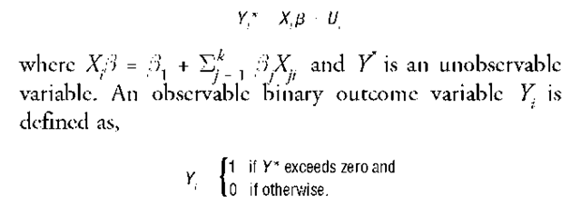
In regression analysis, researchers frequently encounter qualitative variables, especially in survey data. A person’s decision to join a labor union or a homemaker’s decision to join the workforce are examples of dichotomous dependent variables. Dichotomous variables also appear in models due to nonobservance of the variable. In general, a dichotomous variable model can be defined as,
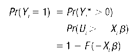
Substituting Y. for Y. and estimating the model by OLS is unsuitable primarily because X. [ represents the probability Y= 1 and it could lie outside the range 0 to 1. In the probit and logit formulations of the above model, the probability that Y. is equal to 1 is defined as a probability distribution function,
where F is the cumulative distribution function of U. The choice of the distribution function F translates the regression function X.ft into a number between 0 and 1. Parameters of the model are estimated by maximizing the likelihood function,
Choosing the normal probability distribution for F yields the probit model, and choosing the logistic distribution for F gives the logit model where P (Y = 1) is given by,
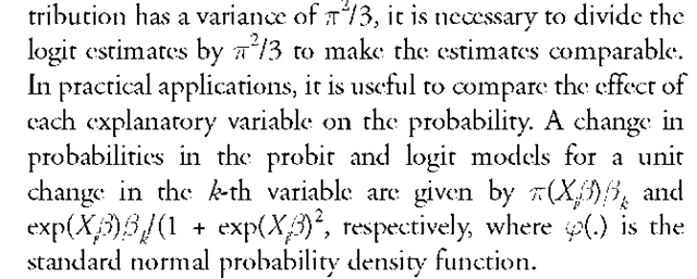
where #(.) is the cumulative normal distribution function. Many statistical packages have standard routines to estimate both probit and logit models. In the probit model, the ft parameters and a appear as a ratio, and therefore cannot be estimated separately. Hence, in the probit model, a is set to 1 without any loss of generality. The cumulative distributions of logit and normal are close to each other, except in the tails, and therefore, the estimates from both models will not be much different from each other. Since the variance of the normal distribution is set to one, and the logistic dis-
In the multivariate probit models, dichotomous variables are jointly distributed with appropriate multivariate distributions. Likelihood functions are based on the possible combinations of the binary choice variable (Y) values. A practical difficulty in multivariate models is the presence of multiple integrals in the likelihood function. Some authors have proposed methods for simulating the multivariate probabilities; details were published in the November 1994 issue of the Review of Economics and Statistics. This problem of multiple integration does not arise in the multinomial logit model because the cumulative logistic distribution has a closed form.
TOBIT MODEL
The Tobit model can be considered as an extension of the probit and logit models where the dependent variable Y. is observed in the positive range and is unobserved or unavailable in the negative range. Consider the model described in equation (2), where
This a censored regression model where Y. observations below zero are censored or not available, but the X observations are available. On the other hand, in the truncated regression model, both Y. and X observations are unavailable for Y* values below zero. Estimation of parameters are carried out by the maximum likelihood method, where the likelihood function of the model is based on Pr(Y* > 0) and PAY" < 0). When U is normally distributed, the likelihood function is given by,
Unlike the probit model, where a was arbitrarily set to 1, the Tobit model estimates the parameters. In the pro-bit model, only the effect on the probabilities for changes in X values are meaningful to a practitioner. However, in the Tobit model, a practitioner may be interested in how the predicted values of Y. change due to a unit change in one X variable in three possible scenarios of the model,
functions. An extension of the Tobit model with the presence of heteroskedasticity has been proposed by James Powell (1984).
CAUSALITY BETWEEN TIME SERIES VARIABLES
The concept of causality in time series variables was introduced by Norbert Wiener (1956) and Clive W. J. Granger (1969), and refers to the predictability of one variable Xt from its past behavior, another variable Yt, and a set of auxiliary variables Z. In other words, causality refers to a certain type of statistical feedback between the variables. Some variables have a tendency to move together—for example, average household income and level of education. The question is: Does improvement in education level cause the income to increase or vice versa? It is also worthwhile to note that even with a strong statistical relation between variables, causation between the variables may not exist. The idea of causation must come from a plausible theory rather than from statistical methodology. Causality can be tested by regressing each variable on its own and other variables’ lagged values.
A closely related concept in time series variables, as well as in cross-sectional data to a lesser degree, is simultaneity, where the behavior of g (g > 1) stochastic variables are characterized by g structural regression equations. Some of the regressors of these regression equations contain stochastic variables that are directly correlated with the random error term. OLS estimates of such a model produce biased estimates, and the extent of the bias is called simultaneity bias. The implications of simultaneity were recognized long before the estimation methods were devised. Within the regression analysis context, the identification problem has another dimension—that is, whether the difficulty in determining a variable is truly random or not. Moreover, a more serious fundamental question that arises is whether the parameters of a model are estimable.


