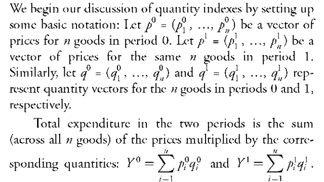
Thus, the ratio of total expenditures in the two periods equals Y / Y 0. If total expenditure is increasing from period 0 to period 1, then Y / Y exceeds 1. If total expenditure is decreasing, then Y VY0 is less than 1. Total expenditure can increase from one period to another simply because prices are increasing. For example, suppose that the quantity vectors are identical in the two periods but the prices of all n goods increase from period 0 to period 1; then total expenditure will also increase.
Quantity indexes can be used to remove the effects of price changes in order to facilitate comparison of expenditures in different time periods. We will use the notation Q01 to denote a quantity index between periods 0 and 1. If the quantity index exceeds 1, then it means that expenditure is increasing from period 0 to period 1 after the effects of price changes have been removed. Similarly, if it is less than 1, then it means that expenditure is decreasing after the effects of price changes have been removed. In the context of national income accounting, quantity indexes can best be thought of as measuring changes in real or inflation-adjusted expenditure; see "How Do I Use Chain-Type Indexes (or Chained Dollar) Measures of Economic Activity, Such as Real GDP?" under FAQs at http://www.bea.gov/index.htm.
A simple and easy-to-interpret way to remove the effects of price changes and, therefore, to calculate a quantity index would be to compare the cost of the quantity vectors in the two periods using a common set of prices. The Laspeyres quantity index, for example, uses the prices
If Q01 exceeds 1, then it means that the period 1 quantity vector costs more than the period 0 quantity vector in period 0 prices. Similarly, if Q^ is less than 1, then it means that the period 1 quantity vector costs less than the period 0 quantity vector in period 0 prices.
The Paasche quantity index is analogous to the Laspeyres quantity index, but with the period 1 prices replacing the period 0 prices. The resulting index is
tors are identical in the two periods, then both Q01 and Q01 will equal 1 even though Yl/Y0 may well differ from 1.
Later, we will develop the concept of superlative quantity indexes, which are preferable to these simple quantity indexes.
PRICE INDEXES, QUANTITY INDEXES, AND THE WEAK FACTOR REVERSAL TEST
Price and quantity indexes are closely related concepts. A price index, P01, is a function of the price and quantity vectors in periods 0 and 1, which measures the change in the prices of the n goods between the two periods. If it is greater than 1, it means that prices increased from period 0 to 1. If it is less than 1, it means that prices decreased.
A price index and a quantity index satisfy the weak factor reversal test if the following equation holds: P01Q01 = YV Y0. Weak factor reversal can be used to formalize our interpretation of quantity indexes as removing the effects of price changes in order to facilitate comparison of total expenditure in two different time periods.
Assume, just for simplicity, that both total expenditure and prices are increasing between the two periods, so
COST OF LIVING, STANDARD OF LIVING, AND SUPERLATIVE INDEXES
Triplett discusses the connection between price and quantity indexes for a set of consumer goods and services and the concept of a cost-of-living index:
A consumption price index should measure the change in the cost of maintaining a fixed, or constant, standard of living. If the price index holds the standard of living constant, then any increase in per capita consumption expenditures that exceeds the increase in the price index can be interpreted as an increase in the standard of living____Thus, from the standard-of-living orientation, the price index measures the changing cost of a constant standard of living, and the quantity index measures increases or decreases in the standard of living. (1992, p. 49)
Diewert (1976) provided a strong rationale for preferring certain price and quantity indexes, which he termed superlative. Without focusing on technicalities, a price index is superlative essentially if it provides a good approximation to the changing cost of a constant standard of living using only the observed price and quantity data. A more extensive discussion of the concept of a cost-of-living index and its connection to superlative price indexes can be found in the entry Price Indices.
A pair of price and quantity indexes is said to be a superlative pair if one of them is a superlative index and the other is defined implicitly by the weak factor reversal test. Thus, for our purposes, it will suffice to interpret a superlative quantity index as one that satisfies the weak factor reversal test in conjunction with a superlative price index (we note, however, that superlative quantity indexes can be defined independently of superlative price indexes without reference to weak factor reversal; see Diewert 1976). In practical terms, following Triplett, this means that superlative quantity indexes can be interpreted as measuring increases or decreases in the standard of living. For an authoritative survey of index number theory, including superlative indexes, see Diewert (1981).
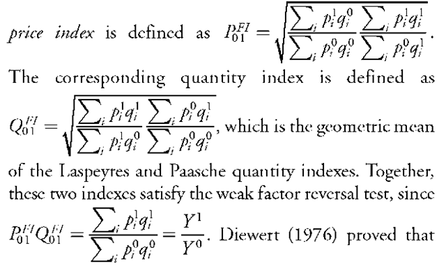
The Laspeyres and Paasche quantity indexes, discussed previously, are not superlative. There are, however, many price and quantity indexes that are known to be superlative. Among these, indexes based on Fisher’s ideal formula have been widely used. Fisher’s ideal
Fisher’s ideal quantity and price indexes are both superlative and, in view of the weak factor reversal test, together they constitute a superlative pair.
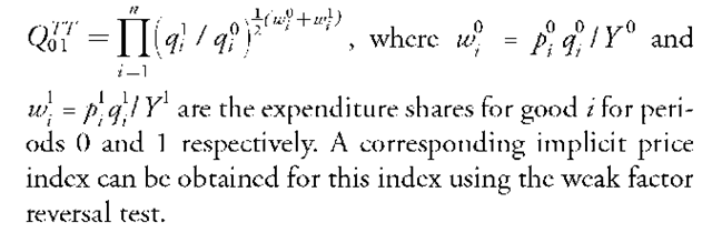
In the same paper, Diewert also proves that the Tornqvist-Theil quantity index is superlative. The Tornqvist-Theil quantity index, Q01", is defined as
CHAIN-WEIGHTING
Suppose that we have price and quantity data for many periods denoted by pt and q, where t = 0, 1, …, T (for example, suppose we have annual data for twenty years). This allows us to compute quantity indexes from each period to the successive one, Q_ 1 , for all t. We can produce a time series covering more than two periods using the concept of chain-weighting. A chain-weighted time series can be constructed as follows: The value of the series, I, for any period t is the previous value of the series, I _ 1, multiplied by the corresponding quantity index for
FROM THEORY TO PRACTICE
National statistical agencies, such as the Bureau of Economic Analysis (BEA), use chain-type quantity indexes to estimate changes in real or inflation-adjusted gross domestic product (GDP) and its components, which can be used when making comparisons over time. BEA (2006) discusses the background and history of the national income and product accounts (NIPAs) for the United States.
As noted by BEA (2006, p. 2), "in 1996, BEA introduced several major improvements to the NIPAs. BEA began estimating the changes in real GDP and its components by chaining together year-by-year quantity changes that were calculated using the Fisher index formula, rather than estimating real GDP on the basis of prices of a single, arbitrary base year." The previous method tended to cause an understatement of real GDP growth for periods prior to the reference year and an overstatement of real GDP growth for periods after the reference year, which is called substitution bias in real GDP growth. These and other problems are eliminated by the use of Fisher’s ideal formula (see BEA 2006, p. 15).
Quantity indexes are useful in other contexts as well. For example, the Federal Reserve Bank of Saint Louis and the Bank of England both produce chain-weighted monetary aggregates based on the Tornqvist-Theil quantity index formula; see Anderson, Jones, and Nesmith (1997) and Hancock (2005), respectively. The Federal Reserve Bank of Saint Louis refers to its superlative monetary aggregates as monetary services indexes, while the Bank of England refers to its as Divisia money. Monetary aggregates include many different types of components—for example, currency, checking accounts, savings deposits, money market mutual funds, time deposits, and the like—which vary in terms of their usefulness for making transactions. As argued by Hancock (2005), Divisia money is a gauge of the money supply that gives the greatest weight to the components of the aggregate that are most used in transactions.
EMPIRICAL ILLUSTRATION
As noted above, the BEA estimates changes in real GDP and its components for the United States by employing chain-type quantity indexes based on Fisher’s ideal formula. In this section, we show how real GDP growth is related to the U.S. business cycle to illustrate the use of quantity indexes.
We obtained the chain-type quantity index for real GDP from BEA and calculated its annualized quarterly growth rate from 1947 to 2006. As identified by the National Bureau of Economic Research (NBER) (see http://www.nber.org/cycles.html) there were ten recessions over the period from 1947 to 2006. These recessions are strongly associated with negative real GDP growth, whereas real GDP growth is usually, although not always, positive when the United States is not in a recession. Annualized quarterly real GDP growth averaged 3.4 percent over the entire period from 1947 to 2006. By comparison, averaging over just the recessionary quarters (peak to trough inclusive) yields average annualized quarterly real GDP growth of — 1.2 percent.
As noted by the Business Cycle Dating Committee of the NBER (2001), the financial press often defines a recession as two consecutive quarters of decline in real GDP. While this is true of most of the recessions identified by NBER, it is not true of all of them.


