19.30.
Reliability may be explicitly defined as the probability that a system will perform satisfactory for at least a given period of time when used under stated conditions. The reliability function is thus same probability expressed as a function of the time period.
Failure is the inability of an equipment to perform its required function. Toe determine the life of a manufactured product for purposes of acceptance inspection, elaborate test apparatus is required to determine the exact moment at which the performance ceases to be satisfactory (or life ends or failure occurs). The definition of satisfactory performance is defined by the specification which depends on the use to which the product is to be put, e.g., a certain product according to one specification may have short life, but long life under another set. In most of the cases, the failure of a component is viewed as terminating its life. In the case of complex manufactured devices where the device can be restored to its original satisfactory performance by replacing one or more components on occurrence of its failures the time expected to elapse between successive failure is important.
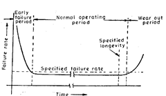
A picture of the failure pattern of certain types of electronic components as well as certain kinds of complex systems is depicted in Fig. 19.33. Initially high failure rates may be expected (premature failures), but on replacement of all the prematurely failing items the failure rate reaches a lower value and then remains fairly constant for very long time (known as normal operating period). During normal operating period the average failure rate remains essentially constant. Most of the acceptance sampling plans, in which case life istiie quality characteristic specified by the designer, are based on the assumption that the failure rate is constant throughout life ; i.e. flat portion of the curve in Fig. 19.33. Obviously, therefore, acceptance sampling can’t be started unless all early premature failures have occurred. Since
generally, the uniform failure rate continues for a longer time than the intended period of use, the final wear out period can be disregarded in the design and interpretation of acceptance sampling plans. Two related quantities used in computing OC curves are failure rate (X’) and arithmetic means or mean life (8′). A.’ is the probability of a failure in a stated unit of time ; unit of time may be any time (one hour is the common practice ; in some instances instead of specifying in hours, it may be
Fig. 19.33. Failure rates vs. time under constant environmental operating conditions.
specified as number of operating cycles in case of switching devices). In the case of complex devices, 0′ is interpreted as the mean time between failures (MTBF). 0′ is also expressed in the same units as used.
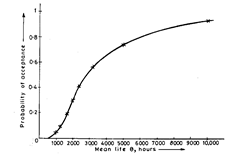
For X’. Considering an acceptance sampling plan based on a stipulated maximum number of test hours, which states : Select 10 items at random from a lot and start testing them. Whenever an item fails, replace it with another item selected at random from the lot. If the test continues for more than 500 hours with not more than 1 failure, accept the lot. If two failures occur before the 500 hours of testing, reject the lot and terminate the test. Obviously, acceptance under this plan requires 10 x 500 = 5000 item hours of test with an acceptance number of 1. If it be assumed that the probability of a failure is the same for every item hour, the OC curve can be calculated in the same way as if it were an ordinary single sampling attributes plant with n = 5000 and c = 1. Here the failure rate X’ takes the place of the fraction defective p’, For life testing plans, the OC curve is plotted in terms of mean life (8′ = 1IX’) rather than in terms of failure rate (X’ corresponding to p’ or ordinary OC curve).
| Failure rate per hour, X’ | Mean life\ours
-h |
Expected average number of failures in 5000 test hours (5000 X) | Probability of acceptance (Probability of one or less failure; Read from Table 19.9) |
| 0.00001 | 100000 | 0.05 | 0.9958 |
| 0.00002 | 50000 | 0.10 | 0.995 |
| 0.00005 | 20000 | 0.25 | 0.974 |
| 0.00006 | 16667 | 0.30 | 0.963 |
| 0.00008 | 12500 | 0.40 | 0.938 |
| 0.00010 | 10000 | 0.50 | 0.910 |
| 0.00020 | 5000 | 1.00 | 0.736 |
| 0.00030 | 3333 | 1.50 | 0.558 |
| 0.00040 | 2500 | 2.00 | 0.406 |
| 0.00050 | 2000 | 2.50 | 0.293 |
| 0.00060 | 1667 | 3.00 | 0.199 |
| 0.00080 | 1250 | 4.00 | 0.092 |
| 0.00100 | 1000 | 5.50 | 0.040 |
It may be noted that the probability of acceptance for a lot that has mean life of 10,000 hours in 0.910 ; or in other words the producer’s risk is 0.09 or 9% of rejecting a lot that has a mean life of 10,000 hours. Similarly the consumer’s risk of accepting a lot that has a mean life of 1,250 hours is 9.2%.
The mean life at various stages in a life test can be estimated by the formula
Fig. 19.34. OC curve for a test of 5000 item hours with acceptance number of 1 (based on assumption of a constant failure rate).
Further if X’ represents a constant probability of failure per hour, then the probability that any one trial will not result in a failure is 1 – X’; and if trials are to be continued until a failure occurs then the theorem of conditional probabilities can be applied to determine the probability of survival, i.e., of no failure and thus the probability of an item surviving for H hours = (1 – X’f*. It may be noted that reliability is also nothing but the probability of no failure throughout some specific period of time.
Reliability = (1 – X’f1 ; and if the value of X’ is very small and H is very large, as is generally the case, then (1 – X’^* can be written = e~m’
The expression e~ HX is usually referred to as exponential reliability function.
If H’ represents the chosen unit time period in hours and P/ is the probability of failure during period H’ the exponential reliability function yields the following formula for mean life in hours :


