Since 1995 there has been an explosion in the exploitation and availability of digital visual media. Digital television and Internet broadcasting continue to merge and viewing figures over the Internet have continued to grow. YouTube/Google and social networking sites have completely changed the way we think about visual media broadcasting while HD television and high-quality mobile displays have changed how often we access and demand content. Therefore the demand for good-quality content has never been higher and hence holders of visual archives (film and video) have found themselves in a completely different commercial landscape for their services as well as their media. Material in archives is generally in poor condition with pictures corrupted by dirt, grain, tearing, and so on. Automated restoration systems provide the only mechanism for exploiting that demand. Before 2000, research in restoration was therefore limited to applications in heritage, but since 2000 a wider commercial requirement has moved automated restoration algorithm development from a fringe activity to an enabling technology in an emerging industry [1]. Companies such as MTIFilm,1 Lowry Digital [1], and Snell and Wilcox2 provide restoration software and hardware, with all post-production houses (e.g., Framestore London, Cinecite UK, ILM) including Dirt Busting software as a matter of course in their arsenal of film treatment tools.
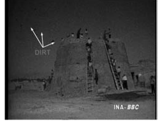
A small subset of defects are illustrated in Figures 11.1-11.6 to show the wide ranging complexity of the problems. Figure 11.1 shows Dirt and Sparkle which occurs when material adheres to the film due to electrostatic effects (for instance) and when the film is abraded as it passes through the transport mechanism. It is also referred to as a Blotch in the literature. The visual effect is that of bright and dark flashes at localized instances in the frame.
FIGURE 11.1
Dirt and Sparkle
FIGURE 11.2
Film Grain Noise is due to the mechanism for the creation of images on film. A piece of dirt is indicated on the image.
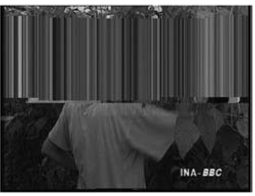
FIGURE 11.3
Betacam Dropout manifests due to errors on Betacam tape.
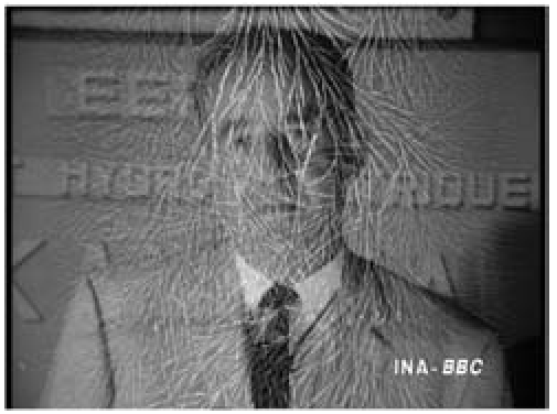
FIGURE 11.4
Vinegar Syndrome often results in a catastrophic breakdown of the film emulsion.
FIGURE 11.5
Kinescope Moire is an aliasing effect.
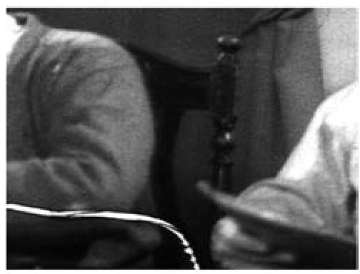
FIGURE 11.6
Film Tear
The image indicates where a piece of Dirt is visible. Figure 11.2 shows Film Grain Noise which is a common effect and is due to the mechanism for the creation of images on film. It manifests slightly differently depending on the different film stocks. The image shows clearly the textured visible effect of noise in the blue sky at the top left. Blotches and noise typically occur together and are the main form of degradation found on archived film and video. A piece of Dirt is indicated on the image. Betacam Dropout (shown in Figure 11.3) manifests due to errors on Betacam tape. It is a missing data effect and several field lines are repeated for a portion of the frame. The repeating field lines are the machine’s mechanism for interpolating the missing data. Vinegar Syndrome often results in a catastrophic breakdown of the film emulsion and is shown in Figure 11.4. This example shows long strands of missing data over the frame. Kinescope Moire (Figure 11.5) is caused by aliasing during Telecine conversion and manifests as rings of degradation that move slightly from frame to frame. Finally, Film Tear in Figure 11.6 is simply the physical tearing of a film frame sometimes due to a dirty splice nearby.
This topic cannot begin to deal in detail with the huge array of algorithms developed for restoration. We instead choose to address the defects that affect the bulk of archived material: Dirt, Lines, Shake, Flicker, and Noise. The reader is given a brief introduction to the principal issues and major results in each case, followed by pointers to more detailed exposition of the algorithms. The topic ends with a discussion of the industry in restoration that has evolved from this body of work.
Dirt and Missing Data
The most common problem in archived film is dirt and sparkle or blotches that manifest as small regions of dark or white pixels. This occurs when film patches have become obscured due to dust or dirt sticking to the film, or completely obliterated due to abrasion of the film material (sparkle). Digital media also suffer from missing data artifacts when bits are corrupted causing loss of blocks or loss of entire frames. Line scratches are also caused by film abrasion and can result in missing data, but often data is still available in the defected area although obscured.
A key difference between missing data as it appears in real footage and speckle degradation is that blotches are almost never limited to a single isolated pixel. Therefore simple spatial order statistic filters with small window sizes cannot remove the distortion, while larger window filters will remove too much detail. Assuming that the missing data does not occur in the same location in consecutive frames, most successful schemes repair the damaged region by copying the relevant information from previous or next frames. This relies on the heavy temporal redundancy present in an image sequence. Because this redundancy is prevalent only along motion trajectories, motion estimation has become a key component of missing data treatment systems.
Historically, the approach has been to develop a method to detect the defect [2], then to correct it by some kind of spatio-temporal interpolation activity [3-6]. The traditional concept in detection is to assume that any set of pixels that cannot be located in next and previous frames must represent some kind of impulsive defect and should be removed. This requires some kind of matching criterion and could be dealt with via a model-based approach [7, 8] or several clever heuristics [7-10]. More complicated systems explore the interaction between the motion estimation and missing data detection/correction stages [11-13].
It is worth mentioning that infrared scans of degraded film have been successfully used for detecting blotches and line scratches. With IR scanners such as [14] the defects show up clearly as patches of grayscale and uncorrupted film regions show up as completely dark. In fact infrared techniques have been recently used to build a ground truth to employ in the objective evaluation of the detection results [15,16]. However, IR can detect image regions which are not perceived as blotches and IR is not suitable if the film medium is not available. This implies that fully digital detection of blotches is still important. In what follows we chart the various solutions up to the present day.
Simple Detection
Consider the simplest image sequence model as follows.
where the luminance at pixel site![]() and the two component motion vector mapping site x in frame n into frame
and the two component motion vector mapping site x in frame n into frame![]() The model error follows a Gaussian distribution
The model error follows a Gaussian distribution The model is therefore consistent with luminance conserving, translational motion in the sequence. The key point here is that image sequences obeying the model show luminance constancy along the motion trajectory. Hence if the backward (for instance) Displaced Frame Difference (DFD) at a pixel site,
![]() is high, there is
is high, there is
probably some defect in the sequence (e.g., missing data) or occlusion/uncovering.
Hence the earliest work on designing an automatic system to “electronically” detect dirt and sparkle flag a pixel as missing if the forward and backward pixel difference was high. This was undertaken by Richard Storey at the BBC [9,17] as early as 1983. The natural extension of this idea by incorporating motion was presented by Kokaram around 1993 [2,7] that allowed for motion-compensated differences. Hence the very simplest detector of missing data flags a pixel as missing when![]() are the forward and backward motion- compensated frame differences. That detector can be improved dramatically if the sign of the DFD is also taken into account, since we can expect the signs to be the same at sites of corruption. That scheme was called the SDIp (Spike Detection Mask).
are the forward and backward motion- compensated frame differences. That detector can be improved dramatically if the sign of the DFD is also taken into account, since we can expect the signs to be the same at sites of corruption. That scheme was called the SDIp (Spike Detection Mask).
The SDI detectors clearly are not pixelwise smooth, and missing data hardly ever corrupts a single pixel. To solve these problems spatial and temporal information needs to be incorporated into the detector. In 1996, Nadenau and Mitra [10] presented such a scheme, which used a spatiotemporal window for inference: the Rank Order Detector (ROD). It is generally more robust to motion estimation errors than any of the SDI detectors although it requires the setting of three thresholds. It uses some spatial information in making its decision. The essence of the detector is the premise that blotched pixels are outliers in the local distribution of intensity.
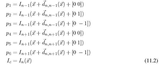
Defining a list of pixels as follows,
where Ic is the pixel to be tested, the algorithm may be enumerated as follows.
1. Sort P1 to p6 into the list where r1 is minimum. The median of these pixels is then calculated as
![]()
2. Three motion-compensated difference values are calculated as follows:
3. Three thresholds are selected t1, t2, t3. If any of the differences exceeds these thresholds, then a blotch is flagged as follows
where The choice of t1 is the most important. The detector works by measuring the “outlierness” of the current pixel when compared to a set of others chosen from other frames. The choice of the shape of the region from which the other pixels were chosen is arbitrary.
Better Modeling
These heuristics have one theme in common. They use some prediction of the underlying true image, based on information around the site to be tested. The difference between that prediction and the observed value is then proportional in some way to the probability that a site is corrupted. In the SDIp, the prediction is strictly temporal. In the ROD the prediction is based on an order statistic; other approaches use morphological filters to achieve the same goal. Poor predictions imply high probability of corruptions. Joyeux, Buisson, Decenciere, Harvey, Boukir et al. have been implementing variants of these techniques for film restoration since the mid-1990s [8,18-23]. Joyeux [8] points out that these techniques are particularly attractive because of their low computational cost. This idea is more appropriately quantified with a Bayesian approach to the problem. Since 1993 [2,5,7,12,13,24-27] this approach was adopted not only to detect missing data but also to reconstruct the underlying image and motion field. Reconstruction of the motion field is very important indeed since temporal prediction is highly dependent on correct motion information.
Assume that we can identify missing pixels by examining the presence of temporal discontinuities. To do this, associate a variable s(x) with each pixel in an image. That variable can have six values or states 600, 601, 610. The variable 6 is binary, indicating whether a pixel site is corrupted, 6 = 1, or not, 6 = 0. The remaining digits encode occlusion hence 00 indicates no occlusion, while 01, 10 imply pixels that are occluded in the next and previous frames respectively. Our process for missing pixel detection requires one to estimate s(·), and those pixels with state 6 = 1 are to be reconstructed. The field 6(x) is the missing data detection field. The degradation model is then a mixture process with replacement and additive noise as follows:
where is the additive noise, and
 is a field of random variables that explain the actual value of the observed corruption at sites where
![]()
Three distinct (but interdependent) tasks can now be identified in the restoration problem. The ultimate goal is image estimation (i.e., revealing In(·) given the observed missing and noisy data). The missing data detection problem is that of estimating![]() at each pixel site. The noise reduction problem is that of reducing
at each pixel site. The noise reduction problem is that of reducing![]() without affecting image details. From the degradation model of (11.3) the principal unknown quantities in frame
without affecting image details. From the degradation model of (11.3) the principal unknown quantities in frame![]() and the
and the
model error These variables are lumped together into a single vector
![]() at each pixel site x.
at each pixel site x.
The Bayesian approach infers these unknowns conditional upon the corrupted data intensities from the current and surrounding frames Gn-1(x), Gn (x), and Gn+1 (x). For the purposes of missing data treatment, it is assumed that corruption does not occur at the same location in consecutive frames, thus in effect![]()
Proceeding in a Bayesian fashion, the conditional may be written in terms of a product of a likelihood and a prior as follows:
This posterior may be expanded at the single pixel scale, exploiting conditional independence in the model, to yield
where denotes the collection of θ values in frame n with
![]() omitted, and C, D, S, denote local dependence neighborhoods around
omitted, and C, D, S, denote local dependence neighborhoods around![]() (in frame n) for variables 6 c, d, and s respectively.
(in frame n) for variables 6 c, d, and s respectively.
Solution
Although that Bayesian expression seems quite complicated, it is possible to exploit marginalization cleverly to simplify the problem at each site and then yield surprisingly intuitive iterative steps. These steps involve local pixel differencing interspersed with simple motion refinement. The key step is to realize that the variables of this problem can be grouped into two sets. The first set contains a pixel state, (defined previously), its associated “clean” image value
![]() and finally the corruption value
and finally the corruption value![]() at each pixel site. The second set contains a motion and error variable
at each pixel site. The second set contains a motion and error variable ![]() for each block in the image. In other words, the variables can be grouped into a pixelwise group
for each block in the image. In other words, the variables can be grouped into a pixelwise group that varies on a pixel grid, and a blockwise group
 , that varies on a coarser grid. Exploiting marginalization we can factor the distributions as follows (using the pixelwise triplet for illustration)
To solve for these unknowns, the ICM (Iterative Conditional Modes) algorithm [28] is used. At each site, the variable set that maximizes the local conditional distribution given the state of the variables around, is chosen as a suboptimal estimate. Each site is visited with variables being replaced with ICM estimates. The maximization is performed through the factorization above, using the marginalized estimate of each variable in turn. Copious details can be found in Kokaram [13] and the reader is directed there for more information.
