This section describes climate change projection methods and results. The projections can be used by urban stakeholders to identify key sector-specific impacts of climate change, as a first step for developing adaptation strategies. The projection component is derived from the global climate models that focus on broad geographical scales, rather than urban climate processes. However, historical data are used for projection baselines, and these baselines reflect the effects of urban climate processes. Some of the challenges of and potential solutions to incorporating urban processes in city-specific climate projections are discussed throughout the section.
Global climate change projection methods
Global climate models
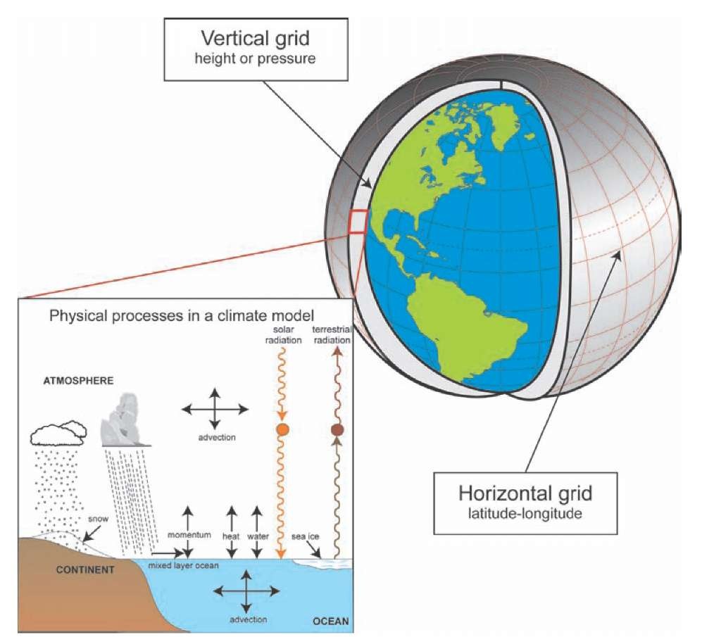
The theoretical impact of atmospheric greenhouse gases on the planet’s energy budget has been recognized since the nineteenth century (Arrhenius, 1896). Global climate models (GCMs) are mathematical representations of climate system interactions that help quantify the impact of greenhouse gases and other system interactions. Climate models also include other climate drivers, including aerosols, land-cover changes, and solar variability. Figure 3.14 depicts physical processes that a climate model simulates.
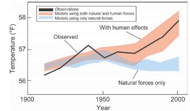
The simulations conducted for the IPCC 2007 report were run at higher spatial resolution than prior simulations and more accurately included complex physical processes such as turbulent fluxes. Current-generation climate models capture many aspects of climate, including twentieth-century warming (when simulated using historical greenhouse gas concentrations and volcanic aerosols) (Figure 3.15). They also capture key climate characteristics of paleoclimates such as the cool Last Glacial Maximum (~21,000 years ago) and warm mid-Holocene (~6,000 years ago). Model successes over a range of historical climate conditions increase confidence that future simulations will be realistic as CO2 concentrations continue to increase.
Figure 3.14: Global Climate Model. Global climate models break the surface down into a series of gridboxes. Within each gridbox, equations are used to simulate the physical processes in the climate system.
Sources of uncertainty: emissions scenarios and climate sensitivity
Despite climate model advances, projections continue to be characterized by large uncertainty (for more information, see Horton et al., 2010). The critical uncertainties concern: • Future concentrations of greenhouse gases and other climate drivers that alter the global energy balance including aerosols and black carbon;
Figure 3.15: Twentieth-century observations and GCM resuts. The observed temperature series follows the model simulation that includes both human effects and natural forces.
• Sensitivity of the climate system to changing concentrations of climate drivers;
• Climate variability, which is largely unpredictable beyond one year in advance, and can mask the climate change signal at urban scales;
• Local physical processes such as the urban heat island, and coastal breezes that occur at smaller spatial scales than GCMs can resolve.
These uncertainties are partially addressed here by using a suite of GCMs and greenhouse gas emissions scenarios, averaged over 30-year time periods to cancel out a portion of the unpredictable natural variability. By presenting the projections as changes through time, uncertainties associated with local physical processes are minimized, although they cannot be eliminated entirely.
Greenhouse gas emissions scenarios
Greenhouse gas emissions scenarios, described in the IPCC Special Report on Emissions Scenarios (SRES; Nakicenovic et al., 2000), are plausible descriptors of possible future socioeconomic, technological, and governance conditions that drive energy demand and fuel choices (Parson et al., 2007). The greenhouse gas concentrations associated with each scenario were used as inputs for global climate model simulations. Three greenhouse gas emissions scenarios (A2, A1B, and B1), were selected for use in this topic.
Figure 3.16: Atmospheric CO2 concentrations resulting from three emissions scenarios. Observed CO2 concentrations through 2003, and future CO2 for 2004 to 2100. The table gives the value of the CO2 concentration for each scenario in 2050 and 2100.
Figure 3.16 shows the CO2 concentration associated with each of these three SRES scenarios. The three scenarios span a reasonably wide range of concentrations and allow for nominal high-, medium- and low-path CO2 futures.
Greenhouse gas concentrations could exceed the levels in these SRES scenarios, due to increases in human emissions (for example, more rapid economic and population growth) or due to carbon and methane cycle feedbacks. As an example of the latter, increasing Arctic temperatures are leading to accelerated permafrost melting, which could lead to the release of stored methane to the atmosphere. As greenhouse gas emissions and concentrations are monitored in the coming decades, it will be possible to better assess the likelihood of high-end emissions scenarios.
Global climate model selection
From the IPCC climate model database, we selected 16 prominent models that had available output for each of the three emissions scenarios. The selected models and their space resolution are listed in Table 3.3. The outputs are collected by the World Climate Research Program (WCRP) and the Program for Climate Model Diagnosis and Intercomparison (PCMDI) (www-pcmdi.llnl.gov/ipcc/about_ ipcc.php), at the Lawrence-Livermore Laboratory in Livermore, California.
While it is unlikely that the future will closely follow a single emissions scenario, or that a GCM projection will capture all aspects of the climate system’s response, using a suite of emissions scenarios and climate model simulations increases the probability that the projection range will span the actual future climate outcome. More information about the rationale for this approach, used by the IPCC, can be found in IPCC, 2007.
Table 3.3: IPCCAR4 climate models.
|
Institution |
Model |
Atmospheric resolution (latitude x longitude) |
|
Bjerknes Centre for Climate Research, Norway |
BCCR |
2.8 x 2.8 |
|
National Weather Research Centre, METEO-FRANCE, France |
CNRM |
2.8 x 2.8 |
|
Canadian Center for Climate Modeling and Analysis, Canada |
CCCMA |
3.75 x 3.75 |
|
CSIRO Atmospheric Research, Australia |
CSIRO |
1.9 x 1.9 |
|
Geophysical Fluid Dynamics Laboratory, USA |
GFDL1 |
2.0 x 2.5 |
|
Geophysical Fluid Dynamics Laboratory, USA |
GFDL2 |
2.0 x 2.5 |
|
NASA Goddard Institute for Space Studies |
GISS |
4.0 x 5.0 |
|
Institute for Numerical Mathematics, Russia |
INMCM |
4.0 x 5.0 |
|
Pierre Simon Laplace Institute, France |
IPSL |
2.5 x 3.75 |
|
Frontier Research Center for Global Change, Japan |
MIROC |
2.8 x 2.8 |
|
Meteorological Institute of the University of Bonn, Germany |
MIUB |
3.75 x 3.75 |
|
Max Planck Institute for Meteorology, Germany |
MPI |
1.9 x 1.9 |
|
Meteorological Research Institute, Japan |
MRI |
2.8 x 2.8 |
|
National Center for Atmospheric Research, USA |
CCSM |
1.4 x 1.4 |
|
National Center for Atmospheric Research, USA |
PCM |
2.8 x 2.8 |
|
Hadley Centre for Climate Prediction, Met Office, UK |
HadCM3 |
2.5 x 3.75 |
Model-based probability
Our combination of 16 global climate models and three emissions scenarios produces a distribution of 48 outputs for temperature and precipitation – in essence a "model-based" probability distribution. As described in Horton et al. (2010), future time periods are compared to a 1971-2000 model baseline. Temperature change is expressed as a difference, and precipitation as a percentage change. It should be noted that the model-based probability distribution will differ from the true probability distribution.
Downscaling
Depending on the model, resolution can be as fine as ~75 –100 miles or as coarse as ~250 —275 miles. Changes from the relevant gridbox are applied to observed station data, a procedure known as the Delta Method that corrects for biases over the baseline period caused by factors such as the spatial mismatch between a gridbox and a point location. More sophisticated statistical and dynamical downscaling techniques can apply more localized change projections. While such techniques should be pursued in the future, a host of issues may hinder their utlility. These issues include: the computational cost of dynamical downscaling and the fact that statistical downscaling may be less valid as climate statistics change (Christensen et al., 2007).
Temperature, precipitation, sea level rise, and extreme events climate projections
The climate projections for temperature and precipitation for the 12 cities are presented first. For sea level rise and extreme event projections, more detailed methodologies are provided in a case study format focusing on New York City.
It is important to recognize the uncertainties associated with climate models. Therefore, the direction of change suggested here is as important as the specific numbers, which are not precise. Table 3.4 summarizes the temperature and precipitation projections for each of the cities for three future timeslices. Shown is the middle 67 percent (central range) of the model projections. Graphs showing the projections for each of the cities are shown in Figure 3.17.
Temperature
All cities are projected to see warming, with temperature increases of between 1.5 and 5.0 °C possible by the 2080s. The city expected to see the greatest warming is Toronto, Canada, with projected increase in temperature by the 2080s ranging from 2.5 to 5.0 °C.
Warming is expected to increase with distance from the equator; Toronto, for example, is expected to warm approximately two times as much as Kingston by 2100 under the A2 scenario. Warming is also generally expected to be greater in interior continental regions than in coastal regions, due to the moderating inertial influence of the oceans. This helps explain why more warming is expected in Toronto than London, even though they are at comparable latitudes. In the extra-tropical regions, warming will generally be greatest in winter.


