Run Lengths (Biomedical Image Analysis)

The run-length method13 to classify texture is very popular and widespread in the analysis of biomedical images. A run is a sequence, in a straight scan direction, of pixels with identical image value. The associated run length is the length of the run, usually the number of pixels for the horizontal or vertical scan direction, or the number of pixels multiplied by V2 for a diagonal direction. The notion of run lengths is related to the transmission of telefax data. Since black-and-white telefax pages contain large areas of contiguous white, it is more efficient to transfer the information "120 pixels of white" than actually transmitting 120 white pixels. In this example, 120 would be the length of a white run. On a black-and-white image, black and white runs can be found, and their length distribution characterized in two histograms. Usually, the image is scanned in four directions: 0°, 45°, 90°, and 135°. The remaining four directions have identical histograms, due to symmetry.

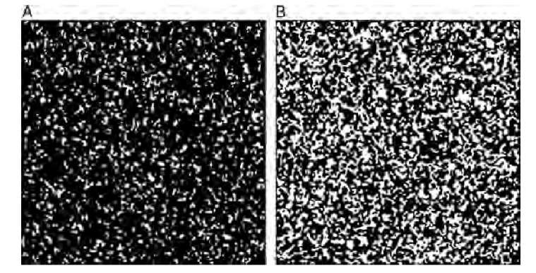
FIGURE 8.12 Test images for demonstration of the run-length method.

Consider the test image in Figure 8.12. The pattern was generated using a cellular automaton algorithm, where a square lattice was filled initially with black pixels and where white pixels were randomly seeded with a probability P. Iteratively, each pixel was set to white when the majority of pixels in its neighborhood (i.e., five or more pixels) were white, and set to black otherwise. Iterations are stopped when the pattern converges. The seeding density was P = 42% in Figure 8.12A and P = 48% in Figure 8.12B. Consequently, Figure 8.12A is dominated by longer black runs compared to Figure 8.12B. The corresponding run-length histograms, scanned in a horizontal direction, are shown in Figure 8.13.

The most obvious difference is the distribution of black runs in Figure 8.12A that is indicated by the broad distribution of the histogram in Figure 8.13A (black line), as opposed to the narrower distribution of black runs in Figure 8.12B (gray line in Figure 8.13A). The distribution of white runs (histogram in Figure 8.13B) is not fundamentally different between the two images in Figure 8.12A and B, although it becomes evident that a larger overall number of white runs exists in Figure 8.12B. If scalar values are needed to describe the texture, the histograms can be further quantified by using the moments of the histogram or by fitting a nonlinear function into the histogram.

The notion of run lengths can be extended to gray-scale images. In gray-scale images, a run extends over pixels with the same gray value. Since this metric is strongly affected by noise and minor intensity fluctuations, it is necessary to quantize the gray-scale values. A run would now be defined as a contiguous sequence of pixels in the scan direction, with pixel intensities falling inside a certain range. If an image has 256 gray levels, it could, for example, be quantized into 16 gray-scale bins, ranging in intensity from 0 to 15, 16 to 31, 32 to 47,…,239 to 255.

FIGURE 8.13 Run-length histograms for the test images in Figure 8.12: (A) the black runs; (B) the white runs.

The optimum bin size depends on the gray-scale variation of the texture. Suitable texture preprocessing (contrast enhancement, background flattening, histogram equalization, and noise reduction) can strongly improve the representation of a specific texture by run lengths. In the case of gray-scale images, the run-length histogram for each scan direction becomes two-dimensional, with one axis being the run length, and the other axis the gray value or gray-value bin. The probability of a specific run length is therefore P(g,l), where g is the gray-value bin and l is the length. If the histogram has been normalized, then

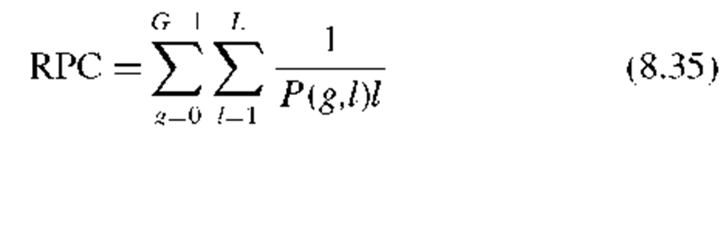
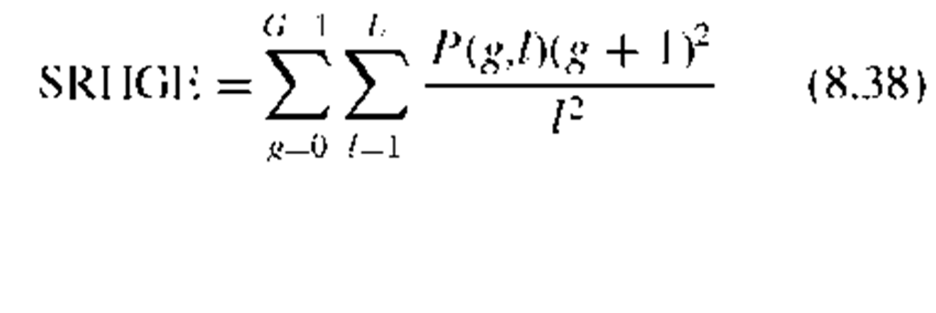
where G is the number of gray-scale bins (the number of bins into which the image has been quantized) and L is the longest run. From the two-dimensional run-length histogram, a feature vector containing seven scalar descriptive values can be extracted. These are commonly known as SRE (short-run emphasis), LRE (long-run emphasis), HGRE (high gray-level emphasis), LGRE (low gray-level emphasis), RLNU (run length nonuniformity), GLNU (gray-level nonuniformity), and RPC (run percentage). In addition, pairwise combinations of short- and long-run emphasis with low and high gray-level emphasis result in the combined values of SRLGE (short-run, low gray-level emphasis), SRHGE (short-run, high gray-level emphasis), LRLGE (long-run, low gray-level emphasis), and LRHGE (long-run, high gray-level emphasis). Equations to compute these quantitative metrics are listed in Table 8.5.

As with all other texture extraction methods, the texture is associated with a multidimensional feature vector suitable for multidimensional thresholding or clustering. Each of the 11 metrics will generally be different for the four directions. The additional information may be used to determine texture anisotropy. For example,in a striated texture (such as the corduroy texture), long runs will be found with a scan direction parallel to the striation, and short runs will dominate the scan direction perpendicular to the striation. In the corduroy example, a higher value for LRE can be expected in the 0° scan direction compared to the 90° scan direction.

TABLE 8.5 Definition of Run-Length Metrics

Description	Equation
Short-run emphasis. This metric increases when short runs dominate, for example, in fine-grained textures.
Long-run emphasis. This metric increases when long runs dominate, for example, in textures with large homogeneous areas or coarse textures.
Low gray-level emphasis. Emphasis is orthogonal to SRE, and the metric increases when the texture is dominated by many runs of low gray value.
High gray-level emphasis. Emphasis is orthogonal to LRE, and the metric increases when the texture is dominated by many runs of high gray value.
Gray-level nonuniformity. This metric increases when gray-level outliers dominate the histogram.
Run-length nonuniformity. This metric increases when few run-length outliers dominate the histogram.
Run percentage. This metric provides information on the overall homogeneity of the histogram and is maximal when all runs are of unity length irrespective of the gray level.
Short run, low gray-level emphasis. This is a diagonal metric that combines SRE and LGRE. The metric increases when the texture is dominated by many short runs of low gray value.
Long run, high gray-level emphasis. This is the complementary metric to SRLGE and increases with a combination of long, high-gray value runs.
Short-run, high gray-level emphasis. This metric is orthogonal to SRLGE and LRHGE and increases when the texture is dominated by short runs with high intensity levels.
Long-run, low gray-level emphasis. Complementary to SRHGE, it increases when the texture is dominated by long runs that have low gray levels.

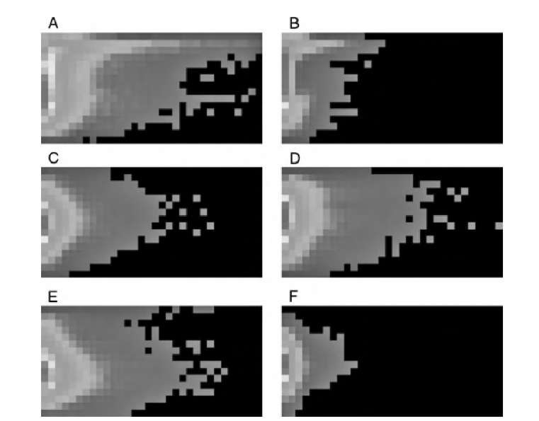
FIGURE 8.14 Run-length histograms of some of the textures in Figure 8.1: (A) corduroy at 0° scan angle, (B) corduroy at 90° scan angle, (C) glass, (D) carpet, (E) bark, and (F) knit, C-F at 0° scan angle. The histograms have been contrast-enhanced and false-colored for better visual representation. Black represents zero; blue low values; green, intermediate values; and red, high values. Each histogram shows increasing gray values (16 bins) from top to bottom and increasing run lengths (32 bins) from left to right.

Gray-scale run-length histograms of some of the textures in Figure 8.1 are shown in Figure 8.14, and some key run-length metrics are given in Table 8.6. It can be seen that the textures are dominated by short runs (large values for SRE). Increased gray-level bins, background flattening, and smoothing would increase the run lengths. The strong anisotropy of the corduroy texture can also be seen. In the vertical direction,short runs dominate and the vertical SRE is almost six times larger than the horizontal SRE, while the horizontal LRE is more than two times larger than the vertical LRE. In addition, the two nonuniformity metrics are much higher in the vertical than in the horizontal direction. The knit texture has values similar to those of corduroy in the vertical direction, but like all other textures, it is more isotropic than corduroy. Bark, carpet, and glass have intermediate values, with bark showing a higher tendency toward longer runs and more uniformity, while glass has shorter runs and more nonuniformity. Each of the rows of Table 8.6 can be seen as a six-dimensional feature vector (i.e., a signature that is specific for the texture).

TABLE 8.6 Run-Length Metrics for the Run-Length Histograms Shown in Figure 8.14

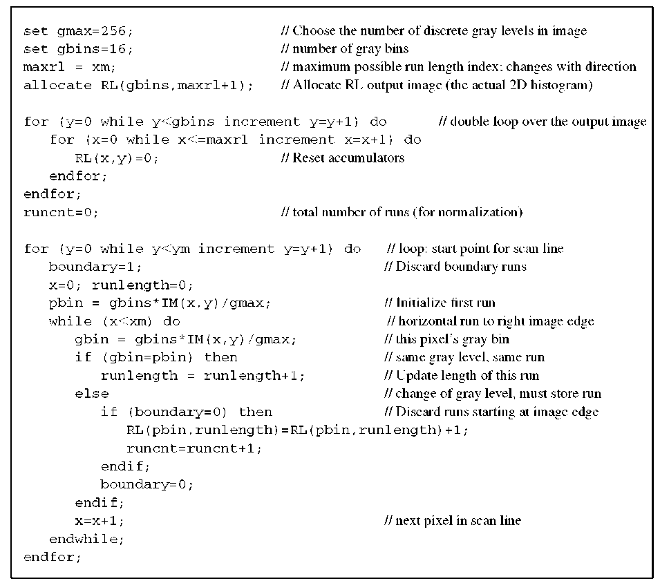
A suggested algorithm to compute the gray-scale run-length histogram can be found in Algorithm 8.3. This algorithm example scans along horizontal scan lines,and each scan line starts at a pixel along the left image edge.

Algorithm 8.3 Run-length histogram for gray-scale images. This algorithm scans along horizontal scanlines. The input image IM(x,y) is a two-dimensional image of size xm and ym and with gmax gray levels. The algorithm produces a two-dimensional histogram RL(g,l), where g corresponds to the gray level and l corresponds to the run length. The variable runcnt contains the total number of runs and can be used to normalize RL to conform to Equation (8.28). The algorithms for 45°, 90°, and 135° are very similar.

To compute the run-length histograms along 45°, 90°, and 135° scan lines, similar functions need to be implemented that differ from Algorithm 8.3 in three aspects. First, the maximum possible run length must be assigned to maxrl. Second, the scan lines start at each pixel of the left and top image edges for 45°, at the top image edge for 90°, and at the top and right image edges for 135°. Third, the while loop needs to be adapted for each scan direction. The algorithm is designed to discard any runs that touch the image edges. Furthermore, the algorithm computes a variable, runcnt, that contains the total number of runs counted. By dividing each element of the output matrix RL by runcnt, the histogram is converted from counts to probabilities. After this normalization, RL conforms to Equation (8.28) and contains the probability of a specific run. This step is required to use RL in the computations of the metrics in Equations (9.29) through (9.39). The implementation of the summations in Equations (9.29) through (9.39) is straightforward by creating a double loop over all elements of RL and adding up the individual elements of RL, weighted with the appropriate factors and powers.