Geoscience Reference
In-Depth Information
(a)
(b)
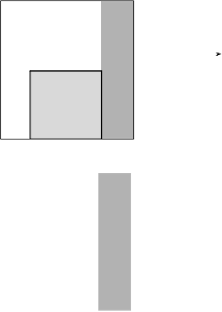
Figure 2.7.
(a) A
three-plate model on a flat
planet. Plate A is
unshaded. The western
boundary of plate B is a
ridge from which seafloor
spreads at a half-rate of
2cmyr
−1
. The boundary
between plates A and C is
a transform fault with
relative motion of
3cmyr
−1
. (b) Relative
velocity vectors for the
plates shown in (a). (c)
The stable solution to the
model in (a): the northern
boundary of plate B is a
transform fault with a
4cmyr
−1
slip rate, and the
boundary between plates
B and C is a subduction
zone with an oblique
subduction rate of
5cmyr
−1
. (d) Vector
addition to determine the
velocity of plate B with
respect to plate C,
C
v
B
.
4
B
v
A
3
Plate A
4
A
v
Plate
C
2
2
3
A
v
3
C
v
A
Plate B
(c)
(d)
3
A
v
Plate A
4
4
Plate
C
3
5
C
v
A
v
CB
5
2
2
Plate B
Cat6cmyr
−
1
. The presence of plate C does not alter the relative motions across
the northern and southern boundaries of plate B; these boundaries are transform
faults just as in Fig. 2.5.Todetermine the relative rate of plate motion at the
boundary between plates B and C, we must use vector addition:
C
v
B
=
C
v
A
+
A
v
B
(2.2)
This is demonstrated in Fig. 2.6(d): plate B is being subducted beneath plate C
at 10 cm yr
−
1
. This means that the net rate of destruction of plate B is 10
=
8cmyr
−
1
;eventually, plate B will be totally subducted, and a simple two-plate
subduction model will be in operation. However, if plate B were overriding plate
C, it would be increasing in width by 2 cm yr
−
1
.
So far the examples have been straightforward in that all relative motions
have been in an east-west direction. (Vector addition was not really necessary;
common sense works equally well.) Now let us include motion in the north-south
direction also. Figure 2.7(a) shows the model of three plates A, B and C: the
western boundary of plate B is a ridge that is spreading at a half-rate of 2 cm yr
−
1
,
the northern boundary of plate B is a transform fault (just as in the other examples)
−
2