Geoscience Reference
In-Depth Information
(a)
(b)
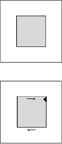
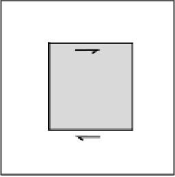
Figure 2.5.
(a) A two-plate
model on a flat planet.
Plate B is shaded. The
western boundary of plate
Bisaridge from which
seafloor spreads at a
half-rate of 2 cm yr
−1
.
(b) Relative velocity
vectors
A
v
B
and
B
v
A
for
the plates in (a). (c) One
solution to the model
shown in (a): the northern
and southern boundaries
of plate B are transform
faults, and the eastern
boundary is a subduction
zone with plate B
overriding plate A. (d) An
alternative solution for the
model in (a): the northern
and southern boundaries
of plate B are transform
faults, and the eastern
boundary is a subduction
zone with plate A
overriding plate B.
4
B
v
A
4
A
v
Plate B
Plate A
(c)
(d)
Plate B
Plate B
Plate A
Plate A
2.2 A flat Earth
Before looking in detail at the motions of plates on the surface of the Earth (which
of necessity involves some spherical geometry), it is instructive to return briefly
to the Middle Ages so that we can consider a flat planet.
Figure 2.3 shows the three types of plate boundary and the ways they are
usually depicted on maps. To describe the relative motion between the two plates
A and B, we must use a vector that expresses their relative rate of movement
(relative velocity). The velocity of plate A with respect to plate B is written
B
v
A
(i.e., if you are an observer on plate B, then
B
v
A
is the velocity at which you see
plate A moving). Conversely, the velocity of plate B with respect to plate A is
A
v
B
, and
A
v
B
=−
B
v
A
(2.1)
Figure 2.3 illustrates these vectors for the three types of plate boundary.
To make our models more realistic, let us set up a two-plate system
(Fig. 2.5(a)) and try to determine the more complex motions. The western bound-
ary of plate B is a ridge that is spreading with a half-rate of 2 cm yr
−
1
. This
information enables us to draw
A
v
B
and
B
v
A
(Fig. 2.5(b)). Since we know the