Geoscience Reference
In-Depth Information
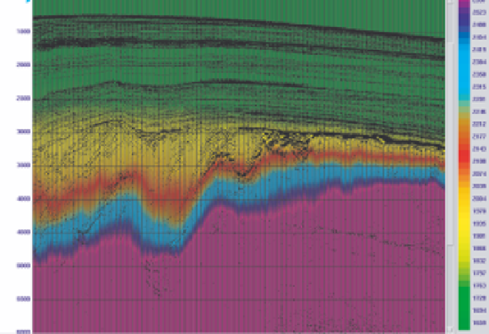
Velocity
(m/s)
TWT
(ms)
Fig. A3.6
Seismic RMS (stacking) velocities (colour) and reflectivity traces.
by applying corrections for measured departure of pore pressure from hydrostatic. For offshore wells,
the compaction trend should use depths below seabed, allowing trends to be compared between wells
in differing water depth. In a similar way, the well density log can be used to establish the density
trend required for the calculation of
S
v
.
The next requirement is the seismic velocity field. How this is created has been explained in
chapter 2
.
Care is needed to get the highest possible accuracy, and pre-stack migration is essential.
A useful check is to apply semi-automatic methods that generate a velocity field for every CMP
gather and display the velocity field together with the reflectivity traces
(fig. A3.6
)
; velocities should
change smoothly across the display in a way that relates to structure. The next step is to convert
these velocities into interval velocities, usually in slabs a few hundred ms thick, using the Dix for-
mula (see
chapter 3
,
section 3.3.3
)
. There is a trade-off between vertical resolution and accuracy
of the interval velocities. For a layer of thickness
h
at depth
D
then the standard error
σ
int
in the
interval velocity due to a standard error
σ
in the picked seismic velocity is given by (Al-Chalabi,
σ
int
=
1
.
4
σ
D
/
h
.
smoothing has been required.
A complication is that we cannot expect the seismic velocities to fit the wells, because of the effect
of anisotropy (
chapter 3
,
section 3.3.3
). Therefore, we need to compare the seismic velocities with
those recorded in the sonic logs of calibration wells within the 3-D survey. It is common to find that
seismic velocities need to be decreased by 5% or so to match the well velocities. Ideally, we would
like to have several calibration wells on the survey to check that the calibration factor is the same at
all of them. If it is, and if they are representative samples of the data volume, then it is reasonable to
assume that anisotropic effects are constant across the area so that a single calibration factor can be
used everywhere. If the calibration factor varies significantly from one well to another, then it may