Geophysical data acquisition, processing and interpretation - Geophysics for the Mineral Exploration Geoscientist - page 48

1 V
+

a)

10 3

0 50

Milliseconds

-

Ch1

Observed
data

10 2

Ch2
Ch3

Ch4
Ch5

Long-wavelength
noise component

10 1

Ch6

Data
after removing
long-wavelength
noise

0

10,000 10,200 10,400

Short-wavelength
noise component

Location (m)

b)

Data after
removing
both long- and
short-wavelength
noise

Total magnetic
intensity
(nT)

Gravity
(gu)

50,400 26

24
22
20
18

50,300

Magnetics

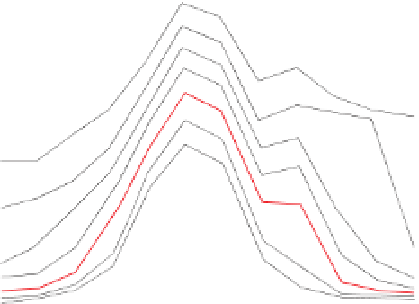
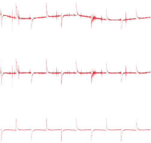
Figure 2.28 Removal of noise from SPECTREM airborne
electromagnetic data to resolve the transient decays using a
variety of

50,200

Gravity

50,100

filtering steps. See text for details. Based on diagrams
in Leggatt et al.( 2000 ) .

Massive sulphide
mineralisation

10,000 10,200 10,400

The enhanced data are obtained from a series of filtering
operations, each treating the data in a different way. This is a
common strategy when working with geophysical datasets.
Some other common combinations of

Location (m)

c)

Resistivity ( m)

n =1

140 60 20 200

filters are gradient

170 300

n =2

76 44 300 500

130 83

filtering of gravity and magnetic data followed by low-pass
filtering to remove the short-wavelength noise enhanced by
the gradient computation, and migration of seismic data
(see Section 6.5.2.5 ) again followed by low-pass filtering to
remove the high-frequency noise that may result.

240

n =3

50 100 78 510

160

130 650

n =4

65 70 410 400

n =5

91 270 670 570

191

740

n =6
Pseudo-depth

140 370

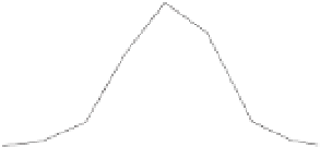
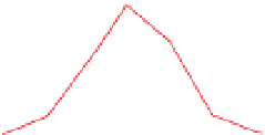
Figure 2.29 Various pro

le plots of geophysical data from the

- - -

Thalanga massive Zn Ag sulphide deposit, Charters Towers,

Queensland, Australia. (a) Electromagnetic data. The various curves
represent the multichannel measurements of the electromagnetic
response at increasing times (channels) after transmitter turn-off. (b)
Gravity and magnetic data. (c) Electrical resistivity pseudosection.
The vertical scale n represents the separation between the source and
receiver located at the surface (see Section 5.6.6.3 ) and is an
indication of the depth influencing the measurement. Based on
diagrams in Irving et al.( 1985 ) .

Pb Cu

2.8 Data display

A variety of techniques are available for displaying 1D and
2D geophysical data, with the different forms of display
emphasising different characteristics of the data. The choice
of display should be made according to the objective of the
interpretation, in particular targeting versus geological map-
ping. The quality of the data is also important, as some forms
of display can be an effective means of suppressing noise.

respectively. Vertical scales are typically linear or logarith-
mic, the later providing amplitude scaling (see Amplitude
scaling in Section 2.7.4.4 ). Often several types of data
are available at each survey location; these may be multi-
parameter measurements or data from different surveys,
and they are plotted together to allow integrated interpret-
ation. Profiles are a simple, accurate and effective way
to display 1D data ( Figs. 2.29a and b ). The most common

2.8.1 Types of data presentation

The simplest form of data presentation is a 1D pro le plot
displaying the variation of a parameter as a function of
distance along a survey traverse, or as a function of time or
frequency for a time- or frequency-based parameter,