Geoscience Reference
In-Depth Information
2
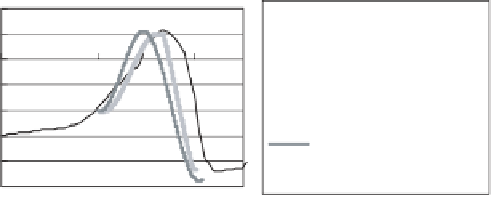
Observation
(Kibedani)
1
0
Simulation
(Dynamical Model,
Kibedani)
Simulation
(Combined Model,
Kibedani)
-1
0
10
20
-2
-3
-4
-5
Time[min]
Fig. 3. Temporal variation of top of a water pole of Kibedani geyser (observation,
simulations dynamical model, Combined model).
6. Comparison between Results of Simulation of the
Combined Model and those of Observation
of Kibedani Geyser
The combined model is first applied to Kibedani geyser because in the case
of it pause modes and spouting modes appear alternately and almost regu-
larly. Results of observation of Kibedani geyser observed by Maeda
et al.
9
were used as comparison with the combined model.
From results of observation of Kibedani geyser we can see a spouting
period is almost 30 min. So at first each parameter has to be decided as a
spouting period
T
30 min using Eq. (4). Moreover, each parameter also
has to be decided as temporal variations of height of top of a water pole of
Kibedani geyser are reproduced by numerical simulations using Eq. (5).
A graph of temporal variations of height of top of a water pole obtained
based on above procedure is shown in Fig. 3. And parameters used by this
simulation of the combined model are as below;
≈
S
=0
.
01 m
2
,
T
e
(temperature of gas in the underground space) = 320 K,
H
= 100 m,
f
k
=22N/m
2
,
V
0
= 990 m
3
,ß=0
.
00019 mol/s.
Above result of simulation is a sample. Possibly another set of param-
eters may bring about more suitable results of simulation. An essential
point is that we can estimate more reliable parameters using the combined
model.
7. Conclusions
We introduced a combined model combining the mathematical model and
the modified dynamical model of a geyser (a periodic bubbling spring)