Geoscience Reference
In-Depth Information
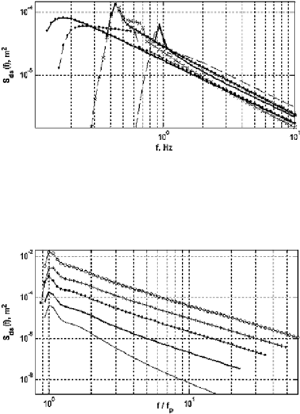
Figure 7.15 Spectral dissipation source function
S
ds
(
f
)
(5.40)
computed with coefficients
a
1
(7.55)
and
a
2
(7.54)
. Computations were performed for Combi spectra
(7.46)
. Different stages of wave
development:
U
10
/
c
p
= 5.7 (bold line), 2.7 (bold line with crosses), 0.83 (bold line with dots), for
wind speed
U
10
=
/
s. Respective wind-input source functions
S
in
(
f
)
are also shown with
plane lines marked with symbols corresponding to the dissipation functions. Figure is reproduced
from
Babanin
et al.
(
2010c
)
10m
©
American Meteorological Society. Reprinted with permission
Figure 7.16 Spectral dissipation source function
S
ds
(
f
)
(5.40)
computed with coefficients
a
1
(7.55)
and
a
2
(7.54)
. Computations were performed for Combi spectra
(7.46)
.Wavesat
U
10
/
c
p
=
2
.
7for
wind speeds
U
10
=
7m
/
s (plain line), 10m
/
s (bold line), 15m
/
s (line with dots), 20m
/
s (line with
crosses) and 30m
/
s (line with circles). Figure is reproduced from
Babanin
et al.
(
2010c
) © American
Meteorological Society. Reprinted with permission
or unimodal directional shapes were assumed for the dissipation source term (see also a
recent study by
Ardhuin
et al.
,
2010
). However, the Lake George experiments (
Young &
Babanin
,
2006a
,see
Section 7.3.6
) revealed that the dissipation function may have symmet-
ric maxima at angles oblique to the main wave-propagation direction. In terms of spectral
modelling, this fact can be interpreted as a bimodal shape of the directional spreading for
the three-dimensional dissipation spectrum. Note that this is a feasibility study only, which
Search WWH ::

Custom Search