Geoscience Reference
In-Depth Information
Line Distance (m)
-7.0
0.1
0.5
1.1
South
3.0
13.0
23.0
33.0
43.0
North
1.4
1.7
2.1
55 mS/m
< 20 mS/m
20-40 mS/m
(a)
> 40 mS/m
70 mS/m
Line Distance (m)
-6.9
South
3.1
13.1
23.1
33.1
43.1 North
0.1
0.5
1.1
1.4
1.7
2.1
35 mS/m
< 20 mS/m
20-40 mS/m
> 40 mS/m
45 mS/m
50 mS/m
(b)
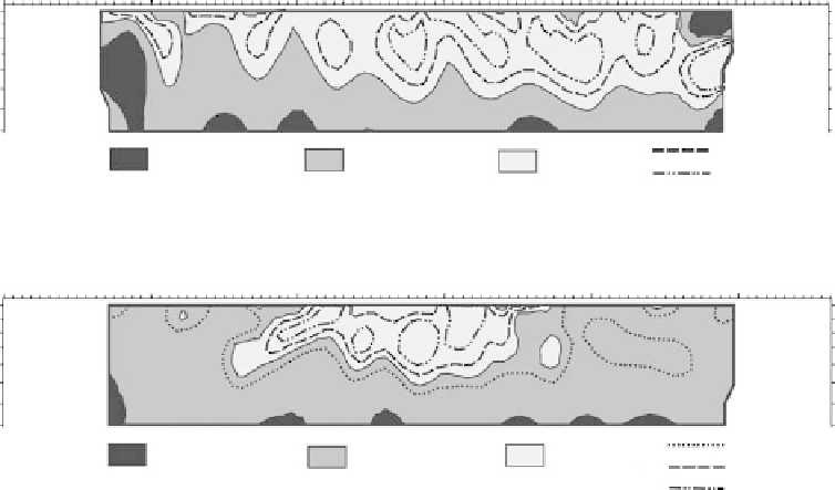
fIGURe 5.15
Two examples of electrical conductivity depth sections.
in Columbus, Ohio. The transect for the Figure 5.15a EC depth section was separated from the
transect for the Figure 5.15b EC depth section by a distance of 41.5 m. Both EC depth sections show
complex EC patterns within the soil profile from the surface down to 2 m. Furthermore, signifi-
cant differences are exhibited among the two Figure 5.15 depth sections even though the distance
between their transects is relatively short. For reference, Figure 5.15b shows EC variations at depth
beneath a south-to-north transect that passes through the center of the test plot where the Figure 5.14
EC
a
map data were obtained.
The data used to produce Figure 5.15a and Figure 5.15b were acquired with the OhmMapper
TR1. The OhmMapper TR1 was configured with a 5 m current dipole and a 5 m potential dipole.
There were four OhmMapper survey passes over each transect corresponding to a depth section on
Figure 5.15. The separation between the current and potential dipoles was increased from 0.625 m
to 1.25 and then to 2.5 m, and again to 5 m for the four successive passes over a transect. Successive
increases in the OhmMapper TR1 dipole-dipole array length provided for greater depths of inves-
tigation. The EC depth sections depicted in Figure 5.15 were generated using the OhmMapper TR1
data as input to a two-dimensional, least-squares optimization inverse computer modeling program,
RES2DINV, developed by Loke (2007). Although not used extensively in agriculture at present,
resistivity (or electrical conductivity) depth sections can potentially provide some very useful agri-
cultural information, such as the vertical position of salinity buildup within the soil profile or the
depth to a clay-pan, fragipan, or caliche layer.
If a number of azimuthal rotation resistivity surveys are carried out within an area of interest,
the results of these surveys could be incorporated into some form of a map product. One possibility
is to plot line segments on a map corresponding to the locations of each azimuthal rotation resistiv-
ity survey. The orientation of a particular line segment on the map would coincide with the principle
axis of the polar graph ρ
a
ellipse, assuming resistivity anisotropy existed at that survey location.
Line segment lengths would in turn reflect ρ
a
-
Max
values. A map such as this could provide valuable
information on the pervasiveness, orientation, and intensity of aligned features present within the
soil profile, for which one example might be the extent, trend, and density of a fracture system.