Geoscience Reference
In-Depth Information
40
35
30
25
20
15
40
35
30
60
42
54
36
25
20
15
48
30
42
10
5
0
10
5
0
24
36
N
30
18
0510 15
Distance (m)
20
25
30
0510 15
Distance (m)
20
25
30
(a)
(b)
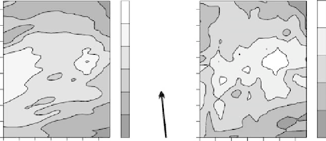
fIGURe 5.14
Apparent soil electrical conductivity (EC
a
) maps of the same agricultural test plot from data
collected with (a) the Veris 3100 Soil EC Mapping System and (b) the OhmMapper TR1. The EC
a
scales for
each map are different, and the EC
a
values are in mS/m.
were collected by the Veris 3100 Soil EC Mapping System (continuous galvanic contact method)
with its 2.1 m electrode array. The data used to produce Figure 5.14b were collected by an Ohm-
Mapper TR1 (continuous capacitively coupled method) with a 5 m current dipole, a 5 m potential
dipole, and a 1.25 m separation between the dipoles. The reported investigation depth for the Veris
3100 with its 2.1 m electrode array is 0.9 m, and the OhmMapper TR1 in the configuration described
had a median investigation depth of 0.8 m. There was an interval of two days between the Veris
3100 and OhmMapper TR1 surveys, but soil temperature and moisture conditions did not change
drastically during this time interval.
When compared to one another, the spatial EC
a
patterns exhibited by both Figure 5.14 maps
appear consistent, and this observation is confirmed by a correlation coefficient (r) between the
two maps that equals 0.79. The average test plot EC
a
from the Veris 3100 survey was 46.5 mS/m,
and the average test plot EC
a
from the OhmMapper TR1 survey was 33 mS/m. The difference in
the average test plot EC
a
may reflect dissimilarities between the Veris 3100 and OhmMapper TR1
systems in regard to the soil volume influencing the instrument response, the magnitude of effects
due to small-scale features, the sensitivity to small changes in field conditions, the relative impact
of unwanted electric signal (noise), procedures for calculating EC
a
, among others. Consequently,
given a particular survey area, the horizontal ρ
a
or σ
a
, EC
a
maps produced with different measure-
ment systems having similar depths of investigation will usually display similar spatial patterns, but
average ρ
a
or σ
a
, EC
a
values may be significantly different. Importantly though, the ρ
a
or σ
a
, EC
a
horizontal spatial patterns prove useful in assessing lateral changes in soil properties.
Two-dimensional resistivity (or electrical conductivity) depth sections characterize the distribu-
tion of resistivity (or electrical conductivity) with depth beneath a measurement transect along the
surface. The resistivity (or electrical conductivity) values shown in a depth section are considered
to represent true values, not apparent values. The data needed to create a depth section can be
obtained several ways, such as through a set of vertical electric soundings conducted at a number
of regularly spaced locations along a transect, several resistivity survey passes over a transect with
a one-electrode array whose length is changed each pass, or one resistivity survey pass over the
transect using several different length electrode arrays at once. The data acquired are then used as
input for the forward or inverse computer modeling programs that generate the resistivity (or electri-
cal conductivity) depth sections.
Two examples of EC depth sections are displayed in Figure 5.15. Each EC depth section is from
a separate agricultural test plot. The two agricultural test plots are situated adjacent to one another