Prediction of Occurrence of Discrete Events - Geomathematics: Theoretical Foundations, Applications and Future Developments - page 167

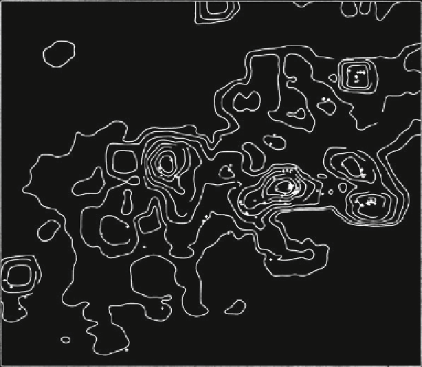
Fig. 5.21 Automatic contour map for occurrence of copper-zinc deposits; linear model applied to
38 lithological variables; contour value represents expected number of (10 km 10 km) cells

containing one or more Cu-Zn deposits per (40 km 40 km) unit area; crosses represent known

Cu-Zn deposits; see Fig. 5.20 for location (Source: Agterberg 1974 , Fig. 3)

made between volcanogenic massive sulphide deposits and magmatic nickel-
copper deposits associated with mafic and ultramafic intrusions.
Following up on Tukey's ( 1972 ) suggestion to use logits, both the linear and
nonlinear model were applied to these two deposit types in the larger study area
with the results shown in Figs. 5.21 , 5.22 , 5.23 , and 5.24 . As before, probabilities
estimated for (10 km 10 km) UTM cells were combined into overlapping unit

cells measuring 40 km on a side to produce estimates of expected values that were
contoured. Comparison of the logistic model pattern of Fig. 5.23 with the linear
model pattern of Fig. 5.21 shows that the two methods gave approximately the same
results for the relatively abundant volcanogenic massive sulphide deposits. On the
other hand, there are significant differences between Figs. 5.22 and 5.24 , which are
for the magmatic nickel-copper deposits that occur rarely in the Precambrian rocks
of the Canadian Shield.
The two types of deposits exhibit different types of geographic distribution
patterns. Ordinary multiple regression could be employed to estimate probability
of occurrence of the massive sulphide deposits but not for the magmatic nickel-
copper deposits because relatively many estimated probabilities were outside the
[0,1] interval. For these relatively rare deposits, logistic regression gave decidedly
better results.