Geoscience Reference
In-Depth Information
Pr = 0.1
Pr = 1
Pr = 7
Pr = 13
Pr = 26
Pr = 50
10
0
10
-1
10
-2
-0.5
0
A
0
0.5 -0.5
0
0.5 -0.5
0
0.5 -0.5
0
0.5 -0.5
0
0.5 -0.5
0
0.5
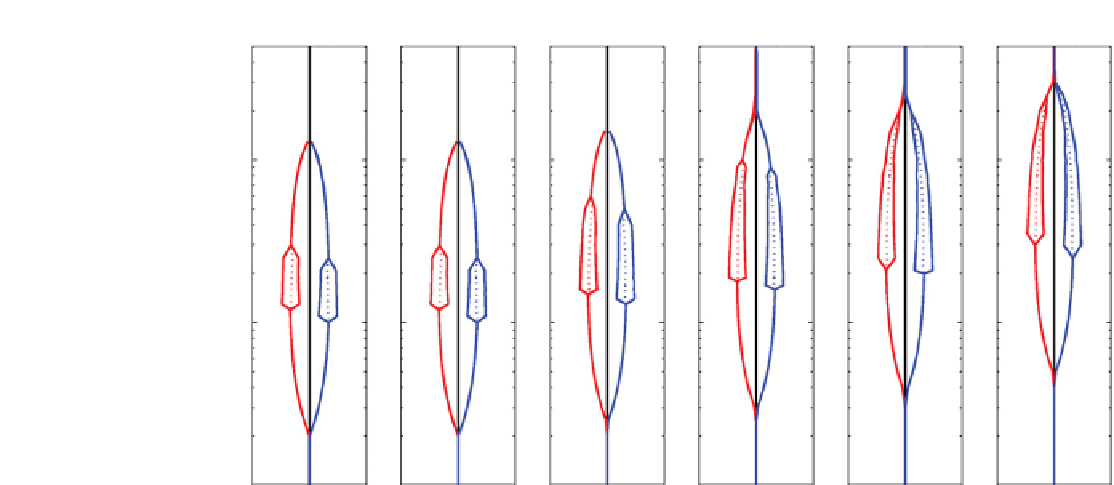
Figure 3.12.
Bifurcation diagrams for Ta = 10
5
and various Prandtl numbers with the thermal Rossby number
as the bifurcation
parameter. The quantity plotted is the amplitude of the mean-flow correction, on the left of the central axis for increasing
and on
the right of the axis for decreasing
. The solid lines indicate the range of the amplitude and the dotted lines the mean amplitude.
affected only slightly since most of the imposed tem-
perature contrast is taken by the thermal boundary lay-
ers. Hence the feedback between sidewall forcing and
baroclinic waves is minor
8. If, on the other hand, the thermal boundary layers
are thicker than the Stewartson layers, the temperature
at the edges of the boundary layers is affected substan-
tially because the baroclinic waves extend to within the
thermal boundary layers and thus provide an additional
heat transfer route across the annulus directly from one
thermal boundary to that at the opposite sidewall.
This principle can be formalized in a one-dimensional
model for the temperature at the interface between the
Stewartson and the fluid interior based on the vertical
heat convection through the Ekman circulation, the radial
heat conduction, and the radial heat convection, which
is a function of the wave amplitude. If the radial extent
of the fluid interior is taken to extend from
y
=
where
v
w
θ
is the heat convection into the interior through
the waves with a radial fluid velocity
v
w
and
w
s
/γ
v
the ver-
tical heat convection through the Stewartson layer with a
vertical velocity
w
s
. The parameter
γ
v
is the vertical aspect
ratio of the annulus. The last term is the horizontal heat
conduction from the wall (at
y
=1+
δ
) to the edge of
the boundary layer (at
y
=1),andfromthatedgetothe
center of the annulus (at
y
= 0). One implicit assumption
here is that the flow and temperature fields are symmet-
ric around the center line. This can then be rearranged
to a differential equation with a constant term, a term
proportional to the effective temperature,
θ
, and a term
proportional to the strength of the baroclinic waves as
quantified by
v
w
,
v
w
θ
∂θ
∂t
=
2
Pr
(
1+
δ)δ
−
2
Pr
δ
−
1
γ
v
−
w
s
.
(3.17)
1 with
y
= 0 at the center of the annulus gap, the
E
1
/
3
layer has
a thickness of
δ
, and the nondimensional temperatures at
the sidewalls are
T
=
±
Coupling this equation to a low-order two-layer model
can then simulate the effect of the now wave-dependent
effective thermal forcing from the edge of the Stewartson
layer. An implementation of this into the minimal
two-layer model of a single wave and a single mean-flow
correction term by
Lovegrove et al.
[2002] is presented
in Appendix B. Some initial results of this are shown as
a set of bifurcation diagrams for a selection of Prandtl
numbers in Figure 3.12, where the Taylor number was
kept fixed at Ta = 10
5
and the bifurcation parameter
was the thermal Rossby number. The diagrams show the
±
1, then the energy equation
∂T
∂t
=
T
+
1
2
T
−
u
·∇
Pr
∇
can be discretized for the temperature at the interface,
T(y)
=
θ
,as
∂θ
∂t
=
v
w
θ
1
−
(
−
1
)
γ
v
)
+
1
(
1
−
θ)/δ
−
θ/
1
−
1
−
w
s
γ
v
−
(
−
Pr
1+
δ/
2
−
1
/
2