Geoscience Reference
In-Depth Information
(a)
(b)
5
0.4
Stable
4
0.3
Lovegrove 2000
3
0.2
2
Holmboe unstable
Williams 2005
0.1
1
KH unstable
0
0
0
1
2
3
4
5
6
0
0.2
0.4
0.6
0.8
k
adim
=
2
π
λ
δ
2
k
adim
=
2
π
λ
δ
2
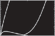
Figure 11.9.
The
k
J
instability diagram for piecewise profiles: (a) experimental areas for interfacial perturbations [
Flór et al.
,
2011] (dashed line) and (b) zoomed in on the regions corresponding to the experiments of
Lovegrove et al.
[2000] and
Williams
et al.
[2005]. The dimensionless wave number
k
=
(
2
π/λ)(δ
v
/
2
)
is based on half the shear thickness
δ
v
/
2.
−
δ
ρ
is not relevant. For the small-scale perturbations in the
experimental fronts under consideration, the wavenumber
and the value of the bulk Richardson number are pre-
sented in the
k
-J diagram in Figure 11.9), where we use
the dimensionless wave number
k
=
(
2
π/λ)(δ
v
/
2
)
based
on half the shear thickness
δ
v
/
2. Apparently, the exper-
imental data fall in the unstable domain of the Hölm-
böe instability, especially in the case of experiments with
immiscible layers [
Lovegrove et al.
, 2000;
Williams et al.
,
2005] for which the validity of the model is optimal.
However, for a two-layer stratified shear flow with mis-
cible layers, a hyperbolic tangent profile with finite thick-
nesses in density and in velocity must be taken into
account for an appropriate approach of a diffusing den-
sity and shear layer (see Figure 11.8b). The variation of
the gradient Richardson number varies drastically with
R
[
Alexakis
, 2005]. As a consequence, the stability diagram
depends also on the thickness ratio (see Figure 11.10).
Moreover, the literature on Hölmböe instability has long
considered the threshold limit of Hölmböe instability at
the value
R
= 2.2 (or even 2.4) and the recent results from
Alexakis show that the location limit is eventually
R
=2.
As illustrated in Figure 11.10 for cases of
R
just above
R
= 2, the unstable Hölmböe domain in the diagram for
the global Richardson number
J
o
=
JR
is very thin and
becomes a line at
R
= 2. Since 1.84
(a)
(b)
2.0
1.5
1.0
0.5
0.0
2.0
1.5
1.0
0.5
0.0
J
KH
J
KH
(c)
(d)
2.0
1.5
1.0
2.0
1.5
1.0
0.5
0.0
0
J
KH
0.5
0.0
J
KH
1
2
Figure 11.10.
Variation of the
k
J
o
diagram (
J
o
=
JR
)asa
function of the thickness ratio
R
(from
Alexakis
[2005]): (a)
R
=4,
(b)
R
=2.5,(c)
R
=2.2,(d)
R
= 2. In (d) the two stability
boundaries (
J
1
and
J
1
S)
have collapsed together on a line and
separate the nonsingular gravity wave modes on the left from
singular neutral modes on the right.
−
For Sc= 700, initially the ratio
R >
2 so that shear insta-
bilities are likely to occur. Indeed, typical Hölmböe waves
(being cusped shaped and with opposite phase direction
below and above the interface) have been observed at the
beginning of the experiments when the density interface
was still relatively sharp (see Figure 11.11).
In the simulations, the ratio
R
is initially large and
subsequently decreases to a critical value close to
R
=2
(see Figure 11.12). Hölmböe instability is therefore pos-
sible but should eventually disappear. When the Schmidt
number is less than 700, the asymptotic value tends to
a value between 1 and 2, suggesting the possibility of
2, i.e.
R
is in
a part of the regime being located under or equal to 2,
it suggests that (in that part of the regime) these small
waves are likely not Hölmböe waves. Indeed, the DNS
simulations confirmed the presence of small-scale pertur-
bations superimposed on the RK mode (Figure 11.12)
that, because of the values of
R
and
J
, could not be due
to stratified shear instability. Since the value of
R
increases
above 2 for Time
>
100 (see Figures 11.7d and also c,e,f),
there will be also a temporal evolution of the stability.
≤
R
≤