Geoscience Reference
In-Depth Information
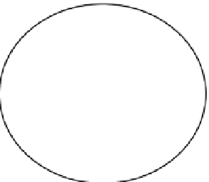
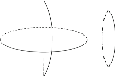
Fig. 6.19 Geometric
description of the UTM
projection
T
1:2
ᄐ
A
1:2
ʳ
1
þ ʴ
1:2
ð
6
:
84
Þ
When converting the triangulation network on the ellipsoid to the Gauss plane,
the grid azimuth on the initial side should be calculated according to (
6.84
). The
geodetic azimuth A
1.2
, according to Laplace's azimuth formula (5.67), can be
obtained through the actually measured astronomical azimuth
ʱ
1.2
, namely:
A
1:2
ᄐ ʱ
1:2
ʻ
1
ð
L
1
Þ
sin
ˆ
1
:
Combining the above two equations, we get:
T
1:2
ᄐ ʱ
1:2
ʻ
1
ð
L
1
Þ
sin
ˆ
1
ʳ
1
þ ʴ
1:2
,
ð
6
:
85
Þ
which is the formula for computing the grid azimuth from the astronomical
azimuth. In (
6.85
),
ʻ
1
and L
1
are the astronomical longitude and geodetic longitude
of P
1
, and
ʳ
1
is the grid convergence of P
1
.
6.6 Universal Transverse Mercator Projection
6.6.1 Definition of UTM Projection
The Gauss projection is also called Transverse Mercator (TM) projection. Geomet-
rically, it can be approximately perceived to be a transverse cylindrical conformal
projection.
The Universal Transverse Mercator (UTM) projection can be understood geo-
metrically as an equiangular transverse secant cylindrical projection. The UTM
system divides the surface of the Earth (considered as a sphere) between 80
S
latitude and 84
N latitude, as shown in Fig.
6.19
. The cylindrical projection
intersects the Earth at two lines (approximate to two meridians). No distortion
occurs anywhere that the projection surface intersects with the Earth's surface. The
scale factor along the central meridian is less than 1.


Search WWH ::

Custom Search