Geoscience Reference
In-Depth Information
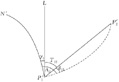
Fig. 6.18 Computation of
grid bearing T
1.2
. The
dashed line indicates the
projected curve
Practical Formula
Equations (
6.78
) and (
6.83
) can both be used as practical formulae for computer
programming to achieve an accuracy of 0.001
00
. The value of B
f
needed to calculate
(
6.83
) can be obtained through iteration or from the direct formula based on x
X.
To reach an accuracy of 0.0001
00
we can expand the series in (
6.83
), and the result is
as follows:
ᄐ
ʳ
00
ᄐ
ρ
00
y
N
f
t
f
ρ
00
y
3
3N
f
þ
ρ
00
y
5
15N
f
t
f
2
f
5t
f
þ
3t
f
þ
2
2
f
t
f
t
f
1
þ
5
ʷ
t
f
2
þ
2
ʷ
f
þ ʷ
:
113
50
0
26.268
00
and B
31
33
0
22.293
00
, according to
For instance, given L
ᄐ
ᄐ
+1
29
0
14.992
00
. Again, given x
(
6.78
) one gets
ʳ ᄐ
ᄐ
3,496,205.167 m and y
ᄐ
+1
29
0
14.992
00
.
269,759.797 m, one obtains from (
6.83
) that
ʳ ᄐ
6.5.5 Computation of Grid Bearing
As shown in Fig.
6.18
, the angle between the curve P
1
0
N
0
and the straight line P
1
0
L
is the
grid co
nvergence
ʳ
1
of point P
1
0
. The angular difference between P
1
0
L and the
chord P
0
1
P
0
2
is the grid azimuth T
1.2
of P
1
0
in the direction of P
1
0
P
2
0
. As the Gauss
projection is conformal, the angle between P
1
0
N
0
and the projected curve P
0
1
P
0
_
(dashed line in Fig.
6.18
) on the plane is equivalent to the angle between P
1
N and
P
1
P
2
on the ellipsoid, which is the geodetic azimuth A
1.2
. From Fig.
6.18
, we have
T
1:2
ᄐ
A
1:2
ʳ
1
ʴ
1:2
j
j:
ʴ
1.2
in Fig.
6.18
is negative. T
1.2
can
therefore be calculated from A
1.2
by applying the formula:
The sign of the arc-to-chord correction
Search WWH ::

Custom Search