Information Technology Reference
In-Depth Information
5
5
5
4
4
4
3
3
3
T
T
v
2
W
2
v
2
W
2
W
2
2
2
2
1
1
1
F''
F''
e
f
e
f
e
f
F'
F'
F'
(
a
)
(
b
)
(
c
)
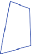
Fig. 2.
Aclose-upofthesituation near inner boundary walk
W
2
.(
a
)Afterdrawing
G
F
around
the tree
T
(heavy dashed line), edges 1
,...,
5 are incident to
v
2
in the correct cyclic order, but
two other edges
e
and
f
pass by between
v
2
and
F
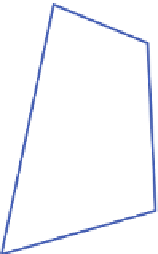
.(
b
) We add a second approximation
F
and
route the edges
e
and
f
(in dashed red) around
W
2
in the buffer zone between
F
and
F
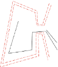
.(
c
)We
route the edges incident to
W
2
in the buffer zone between
F
and
F
.
route these edges around
W
i
using approximations to
W
i
via Lemma 1, and we can do
so in
F
F
. This adds at most
m
W
i
+2 bends to an edge with endpoint on
W
i
;thetwo
additional bends are needed to separate edges at
v
i
,andturn to connect to
W
i
.There
is one difficulty: there are edges of
G
F
that pass by
v
i
, separating it from the segment
of
F
close to
v
i
(which is our gate to
W
i
). To remedy this difficulty, we first route all
of these edges around the whole obstacle
W
i
in the
F
−
−
F
part of the buffer, which
adds
m
W
i
+2bends to an edge every time it passes
v
i
. Now we are free to route the
G
F
-edges incident to
v
i
to their endpoints along
W
i
. Since an edge can pass by and/or
terminate at a vertex at most six times, the total number of additional bends in each edge
caused by going around
W
i
is 6(
m
W
i
+2)
≤
6(
m
F
+2)
≤
18
m
F
+12. Since each
G
F
edge started with 12
n
T
bends, each
G
F
edge now has at most 12
n
T
+18
m
F
+12
bends. Using
m
F
≤
4
n
H
we conclude that each edge has at most 48
n
H
+54
n
H
+ 12 = 102
n
H
+12bends.
Let us now analyze the running time of the algorithm. Most of the steps in the
construction can be performed in linear time. Building the triangulation takes time
O
(
n
H
log
n
H
). The overall running time is thusbounded by the size of the resulting
drawing which contains a linear number of edges each with a linear number of bends,
yielding the quadratic running time.
We conclude the section by proving Lemma 3. Pach and Wenger's[20]algorithm
to draw a planar graph
G
with vertices at fixed locations has three ingredients: (
i
) they
show how to assume that
G
is Hamiltonian, (
ii
) they show how to draw the Hamiltonian
cycle of
G
,and(
iii
), they show how to draw the remaining edges of
G
. In order to prove
Lemma 3, we will follow their structure closely. We will use their result (
i
) directly:
m
H
≤
3
n
H
,and
n
T
≤
m
F
+3
b
−
4
≤
3
m
F
+3
b
−
4
≤
Lemma 4 (Pach, Wenger [20]).
Givenaplanar graph
G
wecan in lineartimecon-
struct a Hamiltonian graph
G
with
E
(
G
)
10
byadding andsubdividing
edges of
G
(each edgeissubdivided byat most two newvertices).
|
|≤
5
|
E
(
G
)
|−