Information Technology Reference
In-Depth Information
v
1
1
5
v
2
W
2
W
1
2
4
3
F'
(
a
)
(
b
)
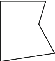
Fig. 1.
A face
F
with outer and inner and boundary walks
W
1
and
W
2
.(
a
)The5edges of
G−H
.
(
b
) The inner approximation
F
(heavy blue lines), a triangulation of it (fine lines), and the dual
spanning tree (dashed red) with extra vertices
v
1
and
v
2
close to
W
1
and
W
2
, respectively.
straight-line drawing of the dual of the triangulation. Bern and Gilbert place a vertex at
the
incenter
of each triangle (where the angle bisectors of the triangle meet) and prove
that the straight-line edge joining two vertices in adjacent triangles lies within the union
of the two triangles. Now take a spanning tree
T
of the dual. For each boundary walk
W
i
,weaugment
T
with a new leaf
v
i
close to
W
i
and inside
F
. This adds
b
vertices to
T
,sothenumber of vertices of
T
is now
n
T
=
m
F
+3
b
4.
Let
G
F
be the embedded multi-graph obtained by restricting
G
to vertices and edges
lying inside or on the boundary of
F
andbycontracting each boundary walk
W
i
of
F
to a single vertex
v
i
. We can now use the following result (extending ideas of Pach and
We nger) to embed
G
F
close to
T
.
−
Lemma 3.
Let
G
be amulti-graphwithagiven planarembedding and fixed locations
for a subset
U
V
(
G
)
of its vertices. Suppose we are givenastraight-linedrawing
of a tree
T
whose leaves include all the vertices in
U
attheir fixed locations. Then
for every
ʵ>
0
there is a planar poly-linedrawing of
G
thatis
ʵ
-close to
T
,that
realizes the given embedding, where the vertices in
U
are attheir fixed locations, and
where each edge has at most
12
n
T
bends. Moreover, each edgeof
G
comes close to
eachvertex in
U
at most six times (where coming close meansentering andleaving an
ʵ
-neighborhood of the vertex or terminating atthe vertex).
ↆ
The proof of Lemma 3 is long and involved, hence we defer it to the end of the
section, and we first proceed with the reminder of the proof of Theorem 1.
We use Lemma 3 to embed
G
F
along
T
so that vertices
v
i
are drawn at their fixed
locations. Each edgeof
G
F
has at most 12
n
T
bends.
We now want to connect edges in
G
F
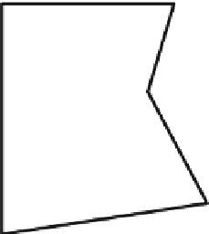
to the boundary components they belong to. We
will use the buffer between
F
and
F
to do this. In fact, we need to split the buffer zone
into two, so we apply Lemma 1 a second time to obtain an inner
ʵ/
2-approximation
F
of
F
,sothat
F
ↆ
F
.SeeFigure 2. The size of the boundary of
F
is at most
3
m
F
(just like
F
). Now for each walk
W
i
we extend the edges ending at
v
i
to their
endpoint on
W
i
. Since we maintained the cyclic order of
G
F
-edges at
v
i
, we can simply
F
ↆ