Image Processing Reference
In-Depth Information
FIGURE 1
Local neighborhood processing with a 3 × 3 filter of an input pixel (
x
,
y
). New pixel
value is stored in the output image at the same coordinates.
Because an operation of local neighborhood in the spatial domain is based on processing the
local and limited area (typically a 3 × 3 or 5 × 5 matrix; also called filter kernel) around every
pixel of the input image, these operations can be implemented separately and independently
for each pixel, which provides the opportunity for these operations to be performed in paral-
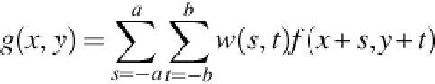
lel. The linear spatial filtering of an image of size
N
×
M
with a filter of size
m
×
n
is defined by
the expression:
where
f
(
x
,
y
) is the input image,
w
(
s
,
t
) are the coefficients of the filter, and
, and
.
The pseudo-code of the algorithm is shown below. An image
f
of size
N
×
M
is being pro-
cessed where a filter
w
of size
n
×
m
is applied, and the result is placed in the output image
g
(see
Pseudo-code 1
)
.
Pseudo-code 1
for
x = 1
to
N
do
for
y = 1
to
M
do
Out = 0;
for
s = -a
to
a
do
for
t = -b
to
b
do
// calculate the weighted sum
Out = Out +
f
(x + s, y + t) * w(s,t)
g
(x,y) = Out
Normally, the filter size is small in size, ranging from 3 × 3 to 5 × 5 matrices. The image size
is, however, could be in thousands of pixels especially when we are working with high-dein-
ition images and video. In the above algorithm, we see four nested loops. However, only the
outer two loops need to be iterated many times; since the inner two loops iterate nine times
total for a 3 × 3 filter. Thus, to speed up performance we need to parallelize the outer two loops
irst, before even considering to parallelize the two inner loops. We can visualize the entire im-


Search WWH ::

Custom Search