Information Technology Reference
In-Depth Information
proc kde
data=nis.diabetesless50los;
univar los/gridl=
0
gridu=
50
method=srot out=nis.kde50 bwm=
3
;
run;
We specify lower (gridl) and upper grid (gridu) values to bound the estimate. The method=srot at-
tempts to optimize the level of smoothness in the estimate. The option, bwm=3, allows you to modify
the optimal smoothness. The 'bwm' stands for bandwidth multiplier. With bwm=3, you take the value
of a
n
computed through the srot method and multiple it by 3 to increase the smoothness of the graph.
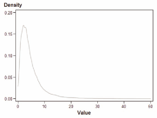
The resulting estimate is saved in the nis.kde50 dataset so that it can be graphed. The result is given in
Figure 5.
The probability is defined as the area under the curve. Most of the probability occurs for a length of
stay between 0 and 10 days, with a much smaller probability of a stay between 10 and 20 days. There
is a very small but nonzero probability of a length of stay beyond 20 days. This probability continues
beyond the value of 50 days. Without the bwm=3 option, the estimate appears more jagged (Figure 6).
Thus, the more jagged curve has the same general appearance compared to the curve in Figure 5.
Therefore, adjusting the bandwidth just gives a better representation of the general pattern of the popu-
lation distribution.
PROC KDE uses only the standard normal density for K, but allows for several different methods
to estimate the bandwidth, as discussed below. The default for the univariate smoothing is that of the
Sheather-Jones plug in (SJPI):
=
{
}
5
7
ò
2
ò
2
hC
fxdx
''( ),
f
'''( )
xdx CKh
(
)
3
4
where C
3
and C
4
are appropriate functionals. The unknown values depending upon the density function
f(x) are estimated with bandwidths chosen by reference to a parametric family such as the Gaussian as
Figure 5. Kernel density estimate of length of stay for patients with diabetes

Search WWH ::

Custom Search