Data Visualization and Data Summary - Text Mining Techniques for Healthcare Provider Quality Determination - page 38

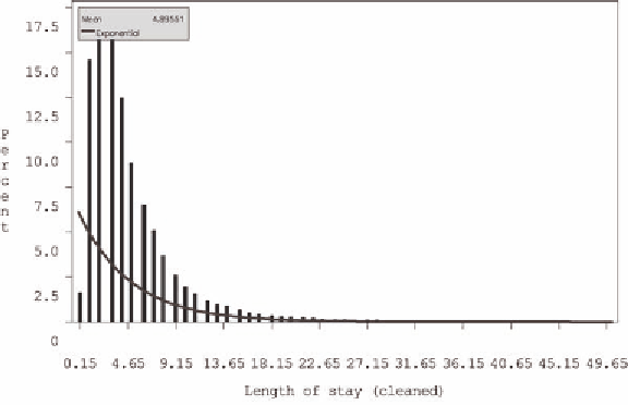
Figure 4. Exponential estimate of population distribution

kernel density estimation

When a known distribution does not work to estimate the population, we can just use an estimate of that
distribution. (Silverman, 1986) The histograms demonstrated in Figures 1-4 can be smoothed into a prob-
ability density function. The formula for computing a kernel density estimate at the point x is equal to

æ ö

xX
a

-

1

n

÷ ÷ ÷ ÷ ÷

ç ç ç ç ç

å

j

fx ()= K

na

è ø

j = 1

n n

where n is the size of the sample and K is a known density function. The value, a n , is called the band-
width. It controls the level of smoothing of the estimate curve. As the value of a n approaches zero, the
curve, f(x) becomes very jagged. As the value of a n approaches infinity, the curve becomes closer to a
straight line.
There are different methods available that can be used to attempt to optimize the level of smoothing.
However, the value of a n may still need adjustments, so SAS has a mechanism to allow you to do just
that. For most standard density functions K, where x is far in magnitude from any point X j , the value of
f(x) will be very small. Where many data points cluster together, the value of the density function will
be high because the sum of x-X j will be large and the probability defined by the kernel function will be
large. However, where there are only scattered points, the value will be small. K can be the standard
normal density, the uniform density, or any other density function. Simulation studies have demonstrated
that the value of K has very limited impact on the value of the density estimate. It is the value of the
bandwidth, a n , that has substantial impact on the smoothness of the density estimate. The true value of
this bandwidth must be estimated, and there are several methods available to optimize this estimate.
The SAS code used to define this function is given below: