Quantification of volcanic reactive halogen emissions - Volcanism and Global Environmental Change - page 124

(a) (b) (c)

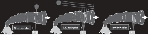
Figure 8.2 Plume scanning schemes: (a) direct light spectroscopy in the UV,
visible or near IR; (b) scattered light spectroscopy in the UV or visible spectral
ranges; and (c) thermal emission is recorded (passive spectroscopy in the thermal
IR). A black and white version of this

figure will appear in some formats. For the
colour version, please refer to the plate section .

where B (

λ

) (with c

¼

speed of light, h

¼

Planck constant, k

¼

Boltzmann constant,
T ¼ temperature) denotes the Planck function and D the optical density as given by
Equation (8.12) . It is interesting to note that the emission spectrum closely resem-
bles the absorption spectrum but, instead of absorption lines (narrow spectral
regions with reduced intensity), emission lines (spectral regions with enhanced
intensity) are seen. Thus, from measurements of the intensity I (

) in the thermal IR
the optical density of a species and (using Equation (8.13) ) its column density can
be determined (see Figure 8.2 ). Note that in practice I (

λ

) frequently has to be
corrected for absorption between the plume and the detector.
Early measurements of CO 2 ,H 2 O and SO 2 by recording their absorption of
direct sunlight were reported by Naughton et al .( 1969 ), more recently also HCl
(Mori et al ., 1993 ) and HF were observed. Passive, IR-emission measurements of
HCl, HF, SiF 4 and SO 2 were e.g. reported by Love et al .( 1998 ). Recently, two-
dimensional distributions of SO 2 and SiF 4 were also measured by passive IR
emission spectroscopy (Stremme et al ., 2012 ).
Independent of the particular spectroscopic technique, the plume scanning
approach usually results in a series of gas column densities S (

λ

α ) as a function of

observation elevation angle (see Figure 8.3 ), i.e. integrals along the line of sight

through the plume as given in Equation (8.12) .
When the distance Y to the plume is known then the angle can be converted to a
lateral distance y

α

α Y across the plume and an integral

ð y 2 ð α 2 ð L

Q ¼ S ð y Þ d y Y c ð x Þ d x d α ð 8 : 16 Þ

y 1 α 0

1

can be calculated. Assuming that the plane of the scan is perpendicular to the
direction of plume motion (if it is not, a simple geometric correction has to be
applied) Q denotes the amount of gas in the cross section of the plume. Finally, the
gas v , where v is the plume propagation

speed, i.e. usually the wind speed at the altitude of the plume.

ux J can be readily calculated as J ¼ Q