Graphics Reference
In-Depth Information
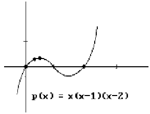
Figure 11.4.
Undesired ripples in interpolating
polynomials.
of d, the closer the curve gets to the segment from
p
1
to
p
2
and the worse the curve
approximates the other segments.
Although Theorem 11.2.1.1 shows that one can always find an interpolating poly-
nomial, there are some serious drawbacks to using this polynomial as the interpolat-
ing curve. First, the degree of the polynomial gets large as n gets large. This would
make it computationally expensive to evaluate. Second, the curve that is generated
will have ripples so that its shape may not match the shape implied by the data. For
example, the unique cubic polynomial that interpolates the points (0,0), (1/3,10/27),
(1/2,3/8), and (2,0) is
()
=-
(
)
(
)
px
xx
1
x
-
,
but its shape has more wiggles than the shape of the polygonal curve through the
points. See Figure 11.4. It is not possible to eliminate the ripples in a polynomial
because an nth degree polynomial always has potentially a total of n - 1 maxima and
minima (up to multiplicity).
11.2.2
Hermite Interpolation
To avoid the polynomial oscillation problem with Lagrange interpolation, one could
piece together polynomials of degree two, but one would in general get corners where
they meet. However, if we try using cubic polynomials, then we have enough degrees
of freedom to force the polynomials to have the same slope where they meet.
11.2.2.1 Lemma.
Given real numbers y
0
, y
1
, m
0
, and m
1
, there is a unique cubic
polynomial p(x) so that
()
=
()
=
¢
()
=
¢
()
=
p
0
y
,
p
1
y
,
p
0
m
,
and
p
1
m
.
0
1
0
1
Proof.
The general cubic
()
=+ +
2
3
px
a bx cx
+
dx
has four degrees of freedom. Substituting our constraints gives four equations in four
unknowns that have a unique solution for the a, b, c, and d.
Alternatively, one can use a matrix approach. Since