Graphics Reference
In-Depth Information
is the probability of such an event, which clearly reflects the volatility inherent in the
business. In addition, it can serve as a useful tool when planning how the insurer's
funds are to be used over the long term.
he ruin probability in a finite time T is given by
ψ
(
u, T
)=
P
inf
<
t
<
T
R
t
<
(
.
)
Most insurance managers will closely follow the development of the risk business
and increase the premium if the business behaves badly. he planning horizon may
be thought of as the sum of the following: the time until the risk business is found to
behave “badly,” the timeuntil the management reacts, andthe time until the decision
to increase the premium takes effect (Grandell,
).
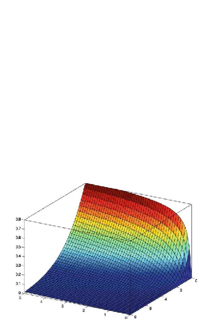
In Fig.
.
, a three-dimensional (
-D) visualization of the ruin probability with
respect to the initial capital u (varying from zero to eight million DKK) and the time
horizon T (ranging fromzero tofive months) isdepicted.he remaining parameters
of the risk process are the same as those used in Figs.
.
and
.
, except that the
relative safety loading was raised from θ
.
. We can see that the
ruin probability increases with the time horizon and decreases as the initial capital
grows.
he ruin probability in finite time can always be computed directly using Monte
Carlosimulations. Naturally, thechoiceofthe intensity function andthe distribution
=
.
to θ
=
Figure
.
.
Ruin probability plot with respect to the time horizon T (let axis,inmonths)andthe
initial capital u (right axis, in million DKK). he relative safety loading θ
.
; other parameters of
the risk process are the same as in Fig.
.
. From the Ruin Probabilities Toolbox
=