Graphics Reference
In-Depth Information
Figure
.
.
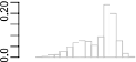
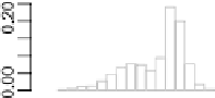
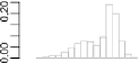
Frequency polygon and variants constructed from the histogram information of Fig.
.
bin origins,
, h
m,
h
m,...,
(
m
−
)
h
m
. he data are prebinned into inter-
vals of width δ
h
m.Letthebincountν
k
denote the number of points in bin
=
B
k
k
δ, kδ
. hen the equally weighted ASH is defined by the equation
=((
−
)
]
m
j
=
m
f
f
j
(
x
)=
(
x
)
x
B
k
.
(
.
)
Using weights w
m
(
i
)
, the weighted ASH becomes
m
j
=−
m
nh
f
x
w
m
j
ν
k
+
j
x
B
k
.
(
.
)
(
)=
(
)
Figure
.
shows the effect of equally weighted averaging of increasing numbers of
histograms for the data and bin width of Fig.
.
.
Kernel Density Estimates
5.1.3
he bin origin can be eliminated altogether by the use of a kernel density estimate.
he result is superior theoretically as well as smoother and thus more appealing vi-
sually.
he estimate requires a smoothing parameter, h, that plays a role similar to that
of the bin width of a histogram and that is sometimes referred to as the bandwidth
of the estimate. It also requires a kernel function, K, which is usually selected to be
a probability density function that is symmetric around
.
From these, the estimator may be written as
n
i
=
n
i
=
nh
x
−
x
i
n
f
(
x
)=
K
=
K
h
(
x
−
x
i
)
(
.
)
h