Graphics Reference
In-Depth Information
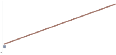
twoway (scatter propval100 popden,
msymbol(S)
)
(lfit propval100 popden,
clwidth(vthick)
)
Note that we add the
msymbol()
option
to the
scatter
command to change the
symbol to a square, and we add the
clwidth()
(connect line width) option
to the
lfit
command to make the line
very thick. When we overlay two plots,
each plot can have its own options that
operate on its respective parts of the
graph. However, some parts of the
graph are shared, for example, the title.
Uses allstates.dta & scheme vg s2c
0
2000
4000
6000
8000
10000
Pop/10 sq. miles
% homes cost $100K+
Fitted values
twoway (scatter propval100 popden, msymbol(S))
(lfit propval100 popden, clwidth(vthick)),
title("This is the title of the graph")
Note that we add the
title()
option
to the very end of the command placed
after a comma. That final comma
signals that options concerning the
overall graph are to follow, in this case,
the
title()
option.
Uses allstates.dta & scheme vg s2c
This is the title of the graph
0
2000
4000
6000
8000
10000
Pop/10 sq. miles
% homes cost $100K+
Fitted values
One of the beauties of Stata graph commands is the way that different graph commands
share common options. If we want to customize the display of a legend, we do it using the
same options, whether we are using a bar graph, a box plot, a scatterplot, or any other
kind of Stata graph. Once we learn how to control legends with one type of graph, we have
learned how to control legends for all types of graphs. Let's look at a couple of examples.
The electronic form of this topic is solely for direct use at UCLA and only by faculty, students, and staff of UCLA.