Graphics Reference
In-Depth Information
twoway (scatter rs id, text( -3 27 "Possible Outliers", size(vlarge)))
(scatteri -3 18 -4.8 10, recast(line))
(scatteri -3 18 -3 3, recast(line)), legend(off)
This graph is similar to the one above
but uses the
text()
option to add text
to the graph. Two
scatteri
commands
are used to draw a line from the text
Possible Outliers
to the markers for
those points. The
coordinates are
given for the starting and ending
positions, and
recast(line)
makes
scatteri
behave like a line plot,
connecting the points to the text.
Uses allstates.dta & scheme vg s2c
yx
Possible Outliers
0
10
20
30
40
50
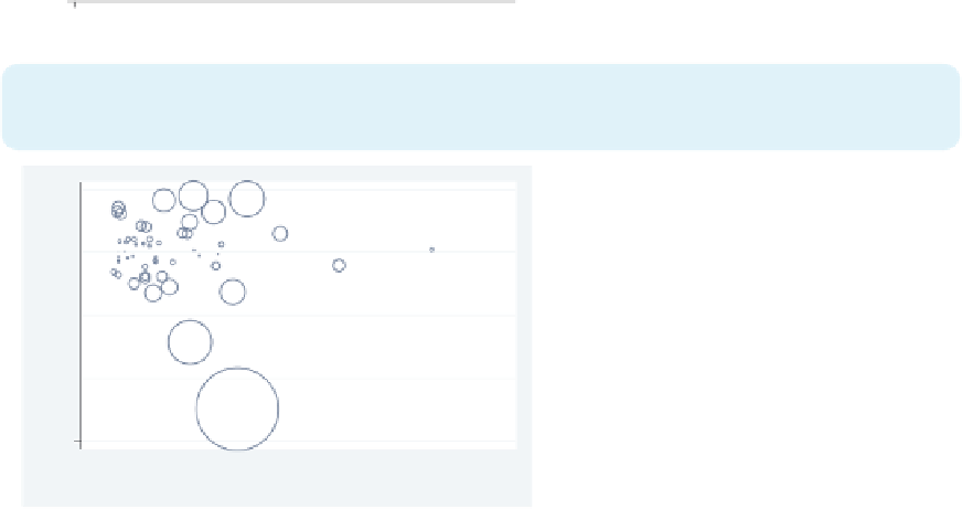
twoway (scatter rs l [aw=cd], msymbol(Oh))
(scatter rs l if cd > .1, msymbol(i) mlabel(stateab) mlabpos(0))
(scatter rs l if cd > .1, msymbol(i) mlabel(cd) mlabpos(6)), legend(off)
This graph shows the
leverage-versus-studentized residuals,
weighting the symbols by Cook's
CT
.1235647
D
(
cd
). We overlay it with a scatterplot
showing the marker labels if
cd
exceeds
.1, with the
cd
value placed underneath.
Uses allstates.dta & scheme vg s2c
AK
.1903994
DC
.6812371
0
.1
.2
.3
.4
Leverage
Imagine that we have a data file called
comp2001ts
that contains variables representing
the stock prices of four hypothetical companies:
pricealpha
,
pricebeta
,
pricemu
,and
pricesigma
, as well as a variable
date
. To compare the performance of these companies,
let's make a line plot for each company and stack them. We can do this using
twoway
tsline
with the
by(company)
option, but we first need to reshape the data into a
long
format. We do so with the following commands:
. vguse comp2001ts
. reshape long price, i(date) j(compname) string
We now have variables
price
and
company
and can graph the prices by company.
The electronic form of this topic is solely for direct use at UCLA and only by faculty, students, and staff of UCLA.