Biomedical Engineering Reference
In-Depth Information
where
x
,
Δx
∈
R
2
or
R
3
are the spatial coordinates and the motion
in those coordinates. Our goal was to find an estimate of the
motion,
ti 103: 50x motion field
30
ˆ
ˆ
t
+
is as close to
I
r
(
x
) as possible.
The similarity between the two images was measured by their
correlation:
x
, such that
I
(
xx
)
20
∑
∑∑
10
I
()()
xx
I
r
t
x
(13. 3)
CI
[(),
xx
I
()]
=
.
(
)
r
t
2
()
2
()
I
x
I
x
0
r
t
x
x
37.5 to 38°C
For motion compensation prior to CBE computation,
ˆ
was
modeled to vary linearly over the image region. Specifically, it
was a linear function of the motion at control points, chosen as
the corners of the 2D image or 3D image volume
-1
-10
0
10
20
30
40
mm
(a)
ti 103: 50x motion field
30
ˆ
x
= …
g
(
x
,
,
x
)
(13.4)
n
ˆ
where
n
is the number of control points. Our goal of finding
x
20
is equivalent to searching for the estimate of
Δx
1
, …,
Δx
n
that
maximizes the correlation function. This procedure is a multi-
variable optimization problem with the correlation as the cost
function
10
0
(
ˆ
ˆ
ˆ
x
,
…=
,
x
)
argmax
CI
[
(),(
xxx
I
+
)].
(13. 5)
1
n
(
x
,
…
,
x
)
r
t
1
n
39.5 to 40°C
-1
-10
0
10
20
30
40
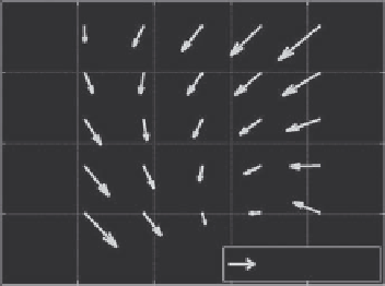
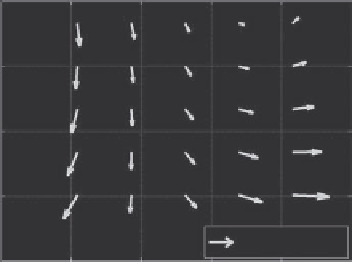
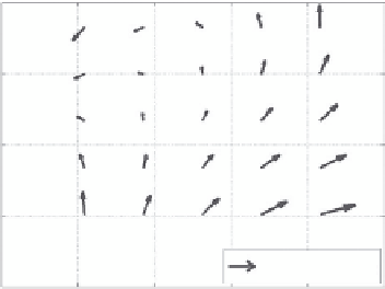
We used the built-in functions in MATLAB
•
to solve this
optimization problem. The motion field over a tissue volume
was represented as a linear function of 3D motion vectors at
eight reference points, the corners of the data volume. Examples
of motion fields in 2D are shown in Figure 13.3 from images
of a live nude mouse.
72
The direction of the arrows represents
the direction of motion; the length of the arrows represents
the magnitude of the motion. It is clear that the motion was
nonrigid.
Our 3D motion-compensation algorithm has been used to
correct for the motion in the images during 3D heating experi-
ments.
73
In each experiment, a sequence of ultrasound RF
images in 3D was obtained at increasing temperature. Motion
between adjacent pairs of 3D image sets was estimated and accu-
mulated relative to the reference image set. Figure 13.4 shows the
3D frame for one specimen of turkey breast muscle, along with
the motion in the axial, lateral, and elevation directions with
temperature at the center slice of the 3D volume.
Accumulated motion in all directions shown in Figure 13.4
was < 340 μm. On average, tissue movement was < 20 μm per
0.5°C step. This small change is consistent with visual observa-
tion of echo shift and apparent motion in images. That displace-
ment is nearly an order of magnitude less than motion tracking
and compensation methods based on correlation can handle in
this application. Displacements for which we compensated took
place over several minutes. Frame intervals for conventional
ultrasound imaging systems can be orders of magnitude smaller.
A typical frame interval is 30 msec. Thus motion between
mm
(b)
ti 103: 50x motion field
30
20
10
0
42.5 to 43°C
-1
-10
0
10
20
30
40
mm
(c)
FIGURE 13.3
Nonrigid motion in 2D in a live nude mouse from (a)
37.5 to 38.0, (b) 39.5 to 40.0, and (c) 42.5 to 43.0°C. Motion is clearly
nonrigid in all three frames. Arrow lengths are 50 times the actual
motion field (similar to Figure 13.5 in Arthur et al.
72
).
frames encountered during clinical applications of ultrasonic
thermometry can be much smaller than we encountered in our
in vitro
studies. Thus frame intervals for thermometry can be
tailored to optimize the effectiveness and speed of motion-com-
pensation algorithms.