Graphics Reference
In-Depth Information
The goodness-of-fit is described by an
energy,
a function that measures how
efficiently the mesh
M
approximates
M
n
as a sum of several terms,
u
v
E
(
M
)=
E
dist
(
M
)+
E
spring
(
M
)+
E
scalar
(
M
)+
E
disc
(
M
)
,
(25.4)
where, for now, we'll combine the last two terms into one,
E
(
M
)=
E
dist
(
M
)+
E
spring
(
M
)+
E
extra
(
M
)
,
(25.5)
which we can ignore for the time being. The “distance” term in the energy is the
sum of the squared distances from each
x
i
to
M
: For each
x
i
, we find the closest
point of
M
(which is itself a minimization problem), square it, and sum up the
results. The “spring” term corresponds to placing a spring along each edge of the
mesh
M
; the rest length of the spring is zero, so the total energy is
E
spring
(
M
)=
(
w
κ
v
i
−
v
j
,
(25.6)
an
edge of
M
v
i
,
v
j
)
where
is a spring constant that we'll describe in a moment. The idea is to adjust
the vertex locations for the mesh
M
to minimize this energy, thus finding a mesh
that fits the data (
X
) well, while not having excessively long edges. Figure 25.22
shows why the spring-energy term is needed.
κ
Figure 25.21: An edge-collapse
can be made gradually, by inter-
polating from the original posi-
tions of u and v part of the way
toward the final position w.
The cost of an edge collapse from a mesh
M
to a mesh
M
is determined by
computing
Δ
E
=
E
(
M
)
−
E
(
M
)
,
(25.7)
which will generally be positive (it's harder to fit the data with fewer vertices!).
Of course, this cost depends on knowing the vertex locations for
M
. Since the
change from
M
to
M
is a single edge collapse, the new knowledge amounts to
just the location of the vertex corresponding to the collapsed edge, since all other
vertices remain unchanged. As we said, Hoppe restricts the possible new vertex
locations for the edge between
v
1
and
v
2
to three choices:
v
1
,
v
2
, and their average.
To compute the distance plus spring cost, he uses an iterative approach, which we
sketch in Listing 25.1.
Listing 25.1: Finding the optimal placement of a vertex for a collapsed edge.
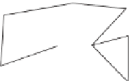
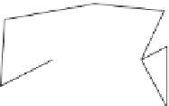
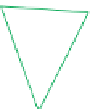
Figure 25.22: The value of
“spring” energy: If we try to fit
the six data points on a circle
(marked with small dots) using
a triangle with short edges, the
green triangle (top) is a reason-
ably good solution. If we remove
the short-edge constraint, the red
triangle (bottom) is a “perfect”
fit, even though it violates our
expectations.
Input: a mesh
M
and an edge
v
s
v
t
of
M
to collapse
Output: the optimal position for
v
s
, the position of
vertex
s
after the collapse
1
2
3
4
5
6
7
8
9
10
11
12
E
←∞
repeat until change in energy is small:
Compute, for each
x
i
∈
X
,
the closest location
b
i
on the
mesh
M
Find the optimal location for location
v
s
by solving a
sparse least-squares problem, using the computed locations
{
b
i
:
i
=
1,
...
K
}
to compute
E
dist
Compute the energy
E
of the resulting mesh
The only difficulty is that the location
b
i
is on the mesh
M
, and it must be
transferred to the mesh
M
; since the two meshes are mostly identical, this is
generally easy. But if
b
i
lies in a triangle containing
v
s
or
v
t
, we compute its