Graphics Reference
In-Depth Information
The idea that “details below the scale of our eyes' ability to detect them don't
matter” can be used in an interesting way: The three colored strips in a typical
LCD display pixel can be individually adjusted in ways that give finer control
than adjusting all three together, even for a grayscale image. For instance, the
antialiased letter “A” shown in Figure 18.14 was originally rendered this way;
Figure 18.59 shows how it looked. This technology, used in font rendering, is
called TrueType [BBD
+
99]. Ideas like this can surely be used in other ways in
graphics as well.
The Nyquist limit, from the discussion in this chapter, appears to be absolute:
You can't sample signals with frequencies above the Nyquist limit and hope to
reconstruct them. But that's not completely true. Suppose that the Nyquist fre-
quency for some sampling rate is
Figure 18.59: Enlarged color
rendering of a black character on
a white background.
ω
0
. Then a signal whose Fourier transform is
nonzero strictly between
ω
0
can be perfectly reconstructed from its sam-
ples. But it's also the case that a signal whose Fourier transform is nonzero strictly
between 5
−ω
0
and
ω
0
can be perfectly reconstructed from its samples,
provided
we know at the time of reconstruction these limits on the transform.
Indeed, if we
know the samples of a function
f
and we know an interval
I
of length 2
ω
0
and 7
1
ω
0
with the
property that
f
's transform is nonzero only strictly within
I
, then we can recon-
struct
f
. Similarly, if we know that the transform of
f
is sparse—that is, nonzero
at relatively few points—we can use this sparsity to reconstruct
f
even if its trans-
form is
not
constrained to an interval of length
0
0
1
ω
0
. This is part of the subject of
the relatively new field of
compressive sensing
[TD06].
1
We started this chapter by saying that every
L
2
function on an interval can
be (nearly) written as a sum of sines and cosines. You might reasonably ask,
“Why sines and cosines? Why not boxes of varying width, or tentlike functions,
or some other collection of functions?” The first answer, which we'll return to in
a moment, is that you
can
write an
L
2
function as a sum of things other than sines
and cosines, and it's often worthwhile to do so. But the Fourier decomposition has
proven widely useful in engineering, mathematics, and physics. Why? One answer
is based on the principle that if you have a linear transformation from a space to
itself, it's often easiest to understand that transformation when you change to a
basis made up of eigenvectors, for then the transformation is just a nonuniform
scaling transformation. Many of the laws of physics appear as second-order linear
differential equations, like
F
=
ma
, in which the unknown position
x
is described
by saying that its second derivative,
a
, must satisfy
F
=
ma
, where the mass
m
and the force
F
are typically known, and
x
is required to satisfy some boundary
conditions as well. In the event that
F
and
m
are constant over time, this is a
second-order equation with constant coefficients. The solutions to such equations
can be generally written as sums of exponentials, where the exponent may be real
or complex. The complex case leads to sines and cosines. Thus, expressing things
as a sum of sines and cosines arises naturally because of the world's defining equa-
tions being second-order linear equations. In fact, Fourier introduced the trans-
form in the process of describing how to solve the
heat equation,
which describes
how the heat in a solid evolves over time in response to initial and boundary
conditions.
Oppenheim and Schaefer [OS09] make a similar case for discrete signals,
saying that every linear shift-invariant system has, as its fundamental solutions,
combinations of sines and cosines.
Shift-invariant
in this context means that if
you regard the system as one that takes an input signal that's a function of
t
and
produces an output signal that's another function of
t
, then delaying the input
0
0
1
1
0
0
1
Figure 18.60: The Haar wavelets
for k
=
0, 1,
and
2
.Fork
>
0
there are
2
k
−
1
basis functions.
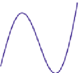
1
0.5
0
0
0.5
1
Figure 18.61: A nice function on
the unit interval.