Graphics Reference
In-Depth Information
(i.e., shifting from
t
→
s
(
t
)
to
t
→
s
(
t
−
h
)
) produces the exact same output, but
shifted by the same amount. In physical terms, it says that the system will behave
the same way tomorrow that it does today.
1
We return now to the first answer—that you
can
write functions as sums of
things other than sines and cosines. Two of the key features of the Fourier decom-
position are localization in frequency and orthogonality. The first means that we
can look at the Fourier transform of a signal and to the degree that the signal is
mostly made up of one frequency, the Fourier transformwill be small except at that
frequency. The second means that the inner product of
exp(
i
n
0.5
0
x
)
is 0 unless
k
=
n
; this means that it's easy to write a function
f
in the Fourier basis
by just computing the inner product of
f
with
exp(
i
n
π
x
)
and
exp(
i
k
π
0
0.5
1
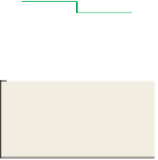
Figure 18.62: An approximation
of the function that's constant on
intervals of size
x
)
for each
n
, and using the
resultant numbers as coefficients in the linear combination.
In his 1909 dissertation under Hilbert, Haar showed that every
L
2
function on
[
0, 1
]
could be well approximated by a sum of functions that were constant on
intervals of size 2
−
k
(for
k
=
0, 1, 2,
π
1
8
.
) and localized in
space,
that is, each func-
tion is nonzero only on two such intervals. These functions (and corresponding
ones for larger
k
) are called the
Haar wavelets.
Figure 18.60 shows a few of the
functions.
Figure 18.61 shows a function
f
on the unit interval, while Figure 18.62
shows an approximation of it that's constant on intervals of length
8
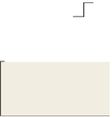
. Figure 18.63
shows how that approximation can be written as a linear combination of the Haar
wavelets: The next-to-bottom row is the weighted sum of the
k
=
3 wavelets, each
portion drawn in a different color; the next up is the sum of the
k
=
2 wavelets,
etc. The top row is a constant function whose value is the average value of
f
on
the interval. The height of the vertical red bar in the bottom row is the sum of the
heights of the red bars in all rows above it.
If we take a limit and approximate the signal by such functions at finer and
finer scales, the coefficients of the resultant (infinite) linear combination is called
the
Haar wavelet transform
of the original function.
While Haar wavelets are conceptually very simple, and share some properties
of the Fourier basis, they lack some others. For instance, they are not infinitely
differentiable; indeed, they're not even once-differentiable. In the mid-1990s, Haar
wavelets, and several other more complex forms of wavelets, with varying degrees
of smoothness, were widely adopted in computer graphics, with applications all
the way from line drawing [FS94] to rendering [GSCH93]. For those who wish
to learn more, we highly recommend
Wavelets for Computer Graphics: A Primer,
by Stollnitz et al. [SDS95], as a gentle introduction to the subject, motivated by
examples from graphics.
By the way, there's an analog to the Shannon theorem for Haar wavelets (or
generally for any other basis in which you choose to write a function): If you have
enough samples of a function that's known to be a combination of a fixed number
of certain basis functions, you can reconstruct the function. For some classes the
locations of the samples may be restricted in various ways (e.g., for Haar wavelets,
they should not be of the form
p
...
1
0
−
1
0
0.5
1
1
0
1
−
0
0.5
1
1
0
1
−
0
0.5
1
1
0
−
1
0
0.5
1
1
0
2
q
, where
p
and
q
are integers), but the general
/
idea still works.
The Fourier basis is a great way to represent one- and two-dimensional signals,
but in graphics we also tend to encounter functions on the sphere, or on
S
2
−
1
0
0.5
1
S
2
,
like the BSDF. There's an analogous basis for
S
2
called
spherical harmonics,
which we touch on briefly in Chapter 31. A nice introduction to these is provided
by Sloan [Slo08].
×
Figure
18.63:
The
approxi-
mation
written
as
a
sum
of
spatially
localized
functions
of
various scales.