Graphics Reference
In-Depth Information
1
that the sample values correspond to various different sinusoids that leads to the
name “aliasing.” In general, if we take 2
N
equispaced samples, then sines of fre-
quency
k
and
k
+
2
N
and
k
+
4
N
, etc., will all have identical samples. But if we
restrict our function
S
to contain only frequencies strictly between
0.5
−
N
and
N
, then
the samples uniquely determine the function. The same idea works for functions
defined on
R
rather than on an interval: If
f
(
0
ω ≥ ω
0
, then
f
can be
reconstructed from its values at any infinite sequence of points with spacing
ω
)=
0for
π/ω
0
.
We can't actually constrain the arriving-light function to not have high fre-
quencies, however. If we photograph a picket fence from far away, the bright
pickets against the dark grass can occur with arbitrarily high frequencies. The
shorthand description of this situation is that “If your scene has high frequencies
in it, then you'll get aliasing when you render it.” The solution is to apply various
tricks to remove the high frequencies before we take the samples (or in the course
of sampling). Doing so in a way that's computationally efficient and yet effective
requires the deeper understanding that the rest of this chapter will give you.
−0.5
−1
0
2
4
6
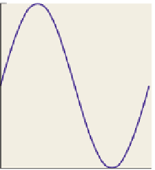
Figure 18.4: Ten evenly spaced
samples of y
=sin(
x
)
on the
interval
[
π
]
.
0, 2
Here's one example of a trick to remove high frequencies, just to give you a
taste. Consider the
sin(
x
)
versus
sin(
11
x
)
example we looked at earlier. We sam-
pled these two functions at certain values of
x
. Let's say one of them is
x
0
. What
would happen if you took your input signal
S
and instead of computing
S
(
x
0
)
, you
computed
3
(
S
(
x
0
)+
S
(
x
0
+
r
1
)+
S
(
x
0
−
1
0.5
r
2
))
, where
r
1
and
r
2
are small random
numbers, on the order of half the sample spacing of 2
10? If the input signal
S
were
S
(
x
)=sin(
x
)
, the three values you'd average would all be very close to
sin(
x
0
)
; that is, the randomization would have little effect (see Figure 18.7). On
the other hand, if the original signal was
S
(
x
)=sin(
11
x
)
, then the three values
you'd average would tend to be very different, and their average (see Figure 18.8)
would generally be closer to zero than
S
(
x
0
)
. In short, this method tends to
atten-
uate
high-frequency parts of the input, while retaining low-frequency parts.
π/
0
−0.5
−1
0
2
4
6
Figure 18.5: The ten samples of
y
=sin(
5
x
)
all turn out to be
zero!
The main ideas we'll use in this chapter are convolution and the Fourier transform,
which you may have encountered in algorithms courses or in the study of various
engineering or mathematics problems.
Fortunately, both convolution and Fourier transforms can be well understood
in terms of familiar operations in graphics; we motivate the mathematics by show-
ing its connection to graphics. Convolution, for instance, takes place in digi-
tal cameras, scanners, and displays. The Fourier transform may be less familiar,
although the typical “graphical display” of an audio signal (see Figure 18.9), in
which the amounts of bass, midrange, and treble are shown changing over time,
shows, at each time, a kind of basic Fourier transform of a brief segment of the
audio signal.
For us, the essential property of the Fourier transform is that it turns convolu-
tion of functions, which is somewhat messy, into multiplication of other functions,
which is easy to understand and visualize.
The Fourier transformation (for functions on the real line) takes a function and
represents it in a new basis; thus, this chapter provides yet another instance of the
principle that expressing things in the right basis makes them easy to understand.
The same tools we use to understand images in this chapter will prove use-
ful not only in analyzing image operations, however: They also appear in the
study of the scattering of light by a surface, which can be interpreted as a kind
1
0.5
0
−0.5
−1
0
2
4
6
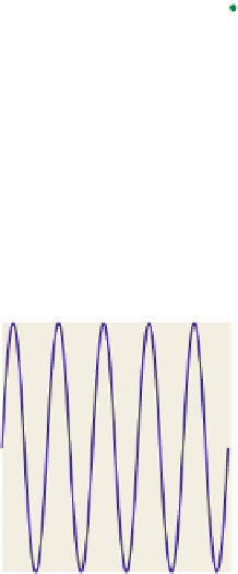
Figure 18.6: The functions x
→
sin(
x
)
and x
→
sin(
11
x
)
have
identical values at our ten sample
points.