Graphics Reference
In-Depth Information
]
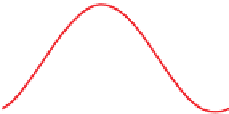
by summing up several periodic
functions on that interval, as shown in Figure 18.1. Surprisingly, we can also (with
the help of some integrals) start with a continuous function
f
on an interval and
break it into a possibly infinite sum of periodic functions, in the reverse of the pro-
cess shown in Figure 18.1. This decomposition is analogous to breaking a vector
in
R
3
into three component vectors along the
x
-,
y
-, and
z
-axes. The coefficients of
the component periodic functions completely determine
f
; the coefficients, listed
in order of frequency, are called the “Fourier transform” of the function
f
. So, if
f
(
x
)=
2.1
cos(
x
)
We can build a continuous function on
[
0, 2
π
2
1
0
−1
8
cos(
3
x
)
, then its Fourier transform, denoted
f
,
is the function with
f
(
1
)=
2.1,
f
(
2
)=
3.5, and
f
(
3
)=
−
3.5
cos(
2
x
)
−
8. (Actually, decompos-
ing the function
f
may involve both cosines
and
sines, but we're going to ignore
this.)
−
−2
Figure 18.1: Summing up peri-
odic functions (in color) of dif-
ferent frequencies leads to more
complicated
The same idea works for functions on the real line: We can take a function
f
:
R
→
R
and compute (with a lot of integration) a different function
f
:
R
→
R
with the property that
f
(
functions,
in
this
ω
)
tells us “how much
f
looks like a cosine of frequency
case the black (thickest) one.
,” just as the
x
-coordinate of a vector
v
in
R
3
tells us how much
v
“looks like”
the unit vector along the
x
-axis. And if you tell me
f
, I can recover
f
from it. So
the
f
ω
f
correspondence gives us two different ways to look at any function:
The first (“the value representation”) tells the value of a function at each point; the
second (“the frequency representation”) tells “how much it looks like a periodic
function of frequency
⇐⇒
ω
” for any
ω
.
5
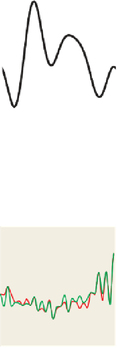
In the course of ray tracing, using one ray per pixel, traced from the pixel cen-
ter, we're taking the function
S
, defined on
R
, and evaluating it at the pixel centers,
which we'll assume are the integer points; that is, we're looking at
S
(
0
)
,
S
(
1
)
,
S
(
2
)
,
etc. It's quite possible for two different functions
S
and
T
to have the same integer
samples (see Figure 18.2). That's reason for concern: The samples we're collect-
ing don't uniquely determine the arriving light! Even so, when we display those
samples on a (one-dimensional) LCD screen, we get a piecewise constant func-
tion (see Figure 18.3) that's not
very
different from either
S
or
T
. And anyhow, our
eyes tend to smooth out the transitions between adjacent display pixels, making
the approximation even better.
0
−5
0
5
10
15
Figure 18.2: The functions S (red)
and T (green) have the same val-
ues at each integer point (black
dots).
How serious a problem is the nonuniqueness of the preceding paragraph? Very.
It's what makes sloping straight lines on a black-and-white display look jagged,
what makes wagon wheels appear to rotate backward in old movies, what makes
scaled-down images look bad, and a whole host of other problems. It's got a name:
aliasing. We'll now see where that name came from by looking at the samples of
some very simple functions: the periodic functions from which all other functions
can be created.
Let's look at the interval
[
0, 2
10
5
π
]
, and consider ten equally spaced samples of
the function
x
sin(
x
)
on this interval, shown in Figure 18.4. From these sam-
ples, it's pretty easy to reconstruct the original sine function. We can come very
close to reconstructing it by just “connecting the dots,” for instance.
The same thing is true for the samples of
x
→
0
→
sin(
2
x
)
or (barely)
x
→
sin(
3
x
)
.
But by the time we look at
x
sin(
5
x
)
(see Figure 18.5), something odd hap-
pens: The samples are all zeroes. By looking at only the samples, we can't tell the
difference between
sin(
5
x
)
and
sin(
0
x
)
. As Figure 18.6 shows, the same is true
for
sin(
1
x
)
and
sin(
11
x
)
.
The means that if our arriving-light function
S
happened to be
x
→
−5
0
5
10
15
Figure 18.3: The light resulting
from displaying samples of either
the red or the green function on a
1D LCD screen, plotted in blue.
sin(
11
x
)
,
we might think, from looking at the recorded samples, that it was
sin(
x
)
instead:
The frequency-11 sine is masquerading as a frequency-1 sinusoid. It's the fact
→