Graphics Reference
In-Depth Information
it's possible for almost every edge to be a contour from some points of view, in
which case forming chains by the obvious greedy algorithm (“search for another
edge that shares this vertex, and add it to my cycle”) can fail badly, generating
contour cycles that intersect transversely, for instance.
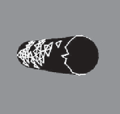
You may object that this example is contrived, but even a randomly triangu-
lated cylinder, when viewed end-on, can have a great many contour edges (see
Figure 34.12). Fortunately, all of these project to the same circle in the final
image, but attempting to make coherent strokes on the contours remains prob-
lematic [NM00].
The problem of multiple contours, and contours that are not smooth, as well
as other artifacts of polygonal contour extraction, are largely addressed by the
work of Zorin and Hertzmann [HZ00], who observe that “no matter how fine the
triangulation is, the topology of the silhouette of a polygonal approximation to
the surface is likely to be significantly different from that of the smooth surface
itself.” They have the insight that the function
g
(
P
)=
n
(
P
)
·
(
P
−
C
)
(34.2)
can be computed at each mesh vertex and interpolated across faces, and then the
zero set of this interpolated approximation of
g
can be extracted and called the
contour. By slightly adjusting the value of
g
at any vertex where it happens to be
zero, they ensure that the contour curves so formed consist of disjoint polygonal
cycles, which are ideal for stroke-based rendering. Figure 34.13 shows an example
of such a contour rendering with “hatching” used to further convey the shape.
We now move on to suggestive contours, ridges, and apparent ridges. To dis-
cuss these features, we must discuss
curvature.
Recall from calculus that the
curvature of the graph of
y
=
f
(
x
)
at the point
(
x
,
y
)
is given by
Figure 34.12: The contours of
a lozenge shape, viewed end-
on, appear to form a circle, but
from a different view they are
quite complex. (Courtesy of Lee
Markosian,
©2000
ACM,
Inc.
Reprinted by permission.)
f
(
x
)
(
1
+
f
(
x
)
2
)
3
/
2
.
κ
=
(34.3)
In the case of a parametric curve
t
→
(
x
(
t
)
,
y
(
t
))
, the formula is
=
x
(
t
)
y
(
t
)
y
(
t
)
x
(
y
)
(
x
(
t
)
2
+
y
(
t
)
2
)
3
/
2
−
κ
.
(34.4)
For a polygonal curve, which is often what we have in practice, there are
simple approximations to these formulas, although you may be better off fitting
the polygonal curve with a spline and then computing the spline's curvature.
Inline Exercise 34.1:
Confirm that if we take the graph
y
=
f
(
x
)
and make
it into a parametric curve using
X
(
t
)=
t
and
Y
(
t
)=
f
(
t
)
, the two curvature
formulas agree.
Figure 34.13: A shape whose
contours are rendered via the
Zorin-Hertzmann algorithm, with
interior shading guided by cur-
vature. (Courtesy of Denis Zorin,
©2000 ACM, Inc. Reprinted by
permission.)
For a surface, curvature is slightly more complex. If you think of a point
P
on a cylinder of radius
r
, there are many possible directions in which to measure
curvature (see Figure 34.14): In the direction parallel to the axis, the curvature
is zero, while perpendicular to it, the curvature is 1
/
r
. To measure each of these,
we intersect the cylinder with a plane through
P
containing the normal vector
n
and direction
u
in which we want to measure the curvature. The intersection is a
curve in this plane, whose curvature at
P
we can measure using Equation 34.3 or
Equation 34.4.