Ionospheric Propagation Effects on GNSS Signals and New Correction Approaches - Global Navigation Satellite Systems: Signal,Theory and Applications - page 400

where a 1 = 2.6123×10 8 , a 2 = 0.8260, a 3 = 6.64. The d I len will be computed in millimeters when β
is measured in radians, f is in MHz, TEC is in TEC units and d 2 TEC / dβ 2 in TECU/deg 2 . The
polynomial coefficients are derived based on a nonlinear fit with ray tracing results in least
square senses.

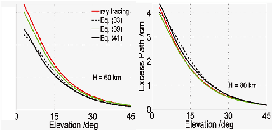
The elevation angle dependence of d I len has been plotted in Fig. 10 using the proposed
correction formula Eq. (41) as well as by Eqs. (33) and (39). In addition, ray tracing results
are plotted for comparisons. Comparing d I len computed by the Eq. (33) and Eq. (41) with ray
tracing results, we see that at higher H values (e.g., H = 80 km) the correction given by the
Eq. (41) performs better. However, its performance degrades at lower H values (e.g., H = 60
km), especially around 7 - 21° elevation angle.

We find that the Eq. (39) gives the best performance. However, it requires ionospheric
parameters H and hm as inputs which are not known to the GNSS users. Inaccurate
assumption of ionospheric parameters may give erroneous estimation of d I len . We see that at
H = 80 km the correction given by the new approach Eq. (41) is even comparable to the
correction given by Eq. (39).

3

ray tracing
Eq. (33)
Eq. (39)
Eq. (41)

4

3

2

2

1

H = 60 km

1

H = 80 km

0 0 15 30 45 0

0 15 30 45

Elevation /deg Elevation /deg

Fig. 10. Comparison of excess path length correction formulas with ray tracing results

While using the proposed correction Eq. (41), it should be remembered that due to its
dependency on the d 2 TEC / dβ 2 term, it is very sensitive to TEC gradients or irregularities. In
such cases the correction given by Eq. (33) is recommended for use.

4.3.2 ΔTEC bend correction
Due to the ray path bending satellite signals propagate in curvature paths instead of straight
LoS paths. However, TECs along a curvature path and the corresponding LoS path are not
the same rather the TEC along the curvature path is slightly larger than the LoS one. The
difference between them is defined as the Δ TEC bend (see Eq. 7). The Δ TEC bend can be
computed by the following formula given by Hoque & Jakowski (2008).