Nonlinear Projections - Transformations and Projections in Computer Graphics - page 145

z

220 0

Be nt

(a) (b)

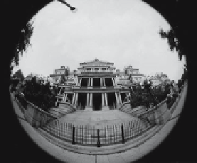
Figure 4.4: (a) Extended Hemispherical Fisheye Projection. (b) Example.

Approximate Hemispherical Fisheye Projection
The downside of the hemispherical fisheye projection is the extensive computations
required by the tangent and arctangent functions. The method described here uses
approximations to simplify the computations. The tradeoff is loss of accuracy, but since
the fisheye projection introduces distortions anyway, many viewers may not be able to
tell accurate results from approximate ones.
Figure 4.2b illustrates the principle. Each point P on the infinitely large circle
corresponds to an angle θ and is moved toward the origin such that its new angle is θ/ 2.
Thus, we can compute the radii of several concentric circles that correspond to, say,
θ =22 . 5 ◦ ,45 ◦ ,67 . 5 ◦ ,and89 ◦ . Similarly, we can compute the radii of the corresponding
circles (the circles for θ/ 2 values) on the radius- k circle. Figure 4.5 shows an example.

Q *

P *

Q

b

a

P

d

c

k

89 0

D C B A

22.5 0 45 0 67.5 0

Figure 4.5: Approximate Fisheye Projection.

If a point P happens to be located on circle A , it is scaled by moving it to the
corresponding circle a on the radius- k circle. Its scale factor is the ratio r a /r A of the